In the fall of 1947, nine clerks at the National Bureau of Standards spent roughly 120 person-days on desk calculators solving one linear program: Jack Laderman’s team ran George Stigler’s cheapest-adequate-diet problem, 77 foods against 9 nutrient minimums, through the brand-new simplex method. They landed on $39.69 a year at 1939 prices, 24 cents under the estimate Stigler had published in 1945. Until that computation nobody could prove how close his guess had been.
Last summer I built an interactive field guide to linear programming, and the figure at the top of it re-runs that kind of computation on every mouse drag. Grab a constraint line, and a simplex solver compiled to WebAssembly re-solves the program before your finger leaves the trackpad. This post is about the engineering underneath that page, and one decision in particular: I wrote the solver twice, in two languages, and made the two implementations police each other.
If your daily work is gradient descent and scipy, linear programming can read like someone else’s subject. It is closer than that. The exact Wasserstein distance is a linear program, Kantorovich’s transport problem, and the classical algorithm for it is a cousin of the solver in this post, and a scipy.optimize.linprog call in a data pipeline lands on the same mathematics. So I will follow one small program the whole way through, and the corners are where it starts. The Python-versus-Rust timing sits in its own section at the end, because it answers a different question than the rest of the post.
A region with corners
Take the smallest worked example on the site, the sketch this post keeps returning to. A fabricator bay can pour two products, and profit is $3x_1 + 2x_2$. Feedstock allows $x_1 + x_2 \le 4$, press time allows $x_1 + 3x_2 \le 6$, and you cannot pour negative amounts. Each limit cuts the plane in half; keeping the allowed side of every cut leaves a polygon of feasible plans, four corners in this case.
Every plan with the same profit sits on one straight line, and raising the profit slides that line across the plane without turning it. Slide it as far as it will go while still touching the region and it comes to rest against the boundary. A flat line leaving a polygon last touches it at a corner, or along a whole edge in the case of a tie, and an edge has corners at its ends. So if a best plan exists at all, one of the corners is a best plan, and there are only finitely many corners to check. (Regions can also be empty, or open in the direction of profit; two of the recorded fixtures exist to pin exactly those verdicts.)
Checking four corners is nothing. But the diet problem’s region lives in 77 dimensions, corner counts grow exponentially with dimension, and “check the corners” stops being a plan almost immediately. What matters is how many corners a solver actually has to visit. Later on I measure that, on a family of programs built to give the worst possible answer.
Watching one walk
The simplex method, which Dantzig devised in 1947, visits corners the way you would climb stairs: start at one, move to an adjacent corner that improves the objective, stop when no neighbor is better. The bookkeeping happens in a tableau, a matrix that holds every constraint with a slack variable added per row. One move between corners is a pivot, and a pivot makes two choices. The entering column answers “which direction improves profit fastest right now,” read off the objective row. The leaving row answers “how far can I go before some limit stops me”: divide each row’s remaining budget by what the step costs it, and the smallest ratio names the first wall you hit. Then one round of Gauss-Jordan elimination rewrites the tableau in terms of the new corner.
The explainer’s centerpiece scales the fabricator bay up to three products under five named limits: the cargo problem, maximize $x_1 + x_2 + x_3$ subject to $-x_1 + x_2 \le 5$, $x_1 + 4x_2 \le 45$, $2x_1 + x_2 \le 27$, $3x_1 - 4x_2 \le 24$, and $x_3 \le 4$. That walk is the one this post keeps re-solving. The site draws it twice at once: on the left, the feasible region as a wireframe polytope with the path traced corner to corner; on the right, the tableau after each pivot, with an objective staircase climbing 0, 8, 15, 19, 22. Both panels read from the same recorded step.
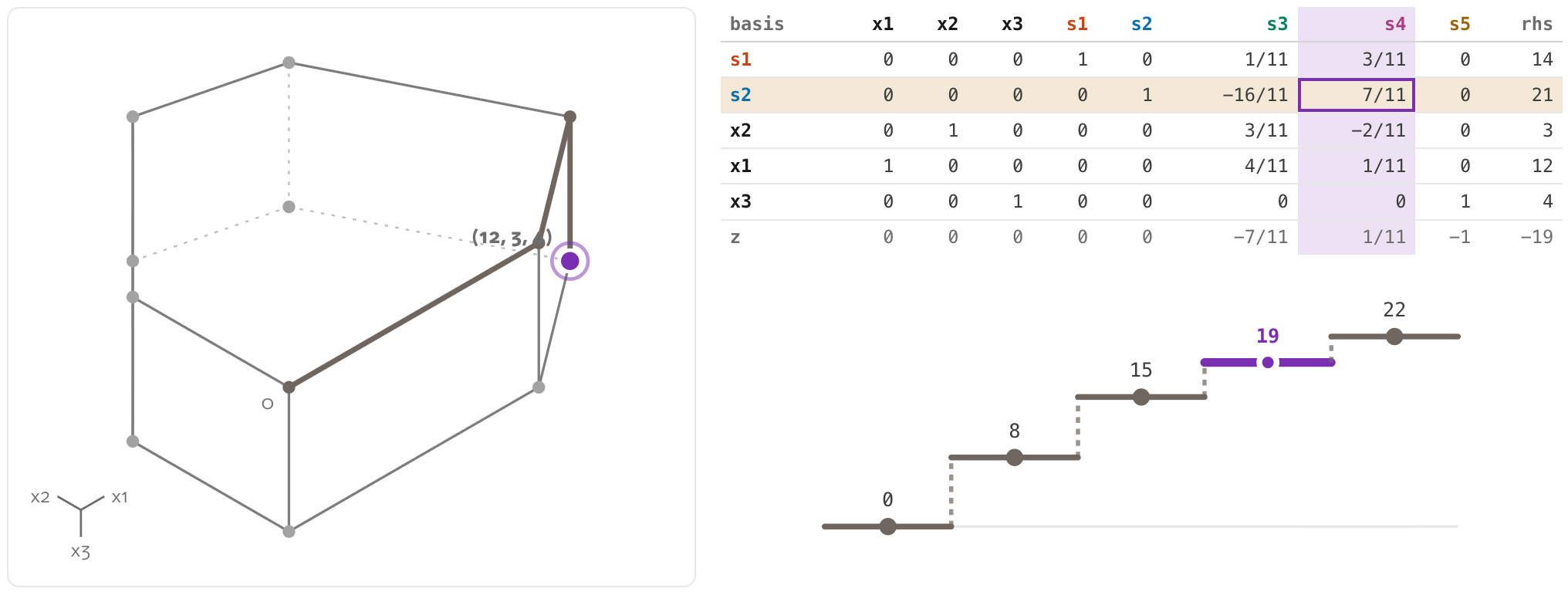
Watch any one of those pivots up close and it is nothing but row reduction: divide the pivot row, clear the column above and below it. “A pivot is row reduction” is the one-line summary I wish I had been handed earlier. It is the elimination from CLRS chapter 28, and chapter 29 builds the whole simplex procedure on top of it.
The bet: write it twice
The figures above are not videos. When a reader drags a limit line, something in the page has to actually re-solve the program, in milliseconds, offline, on whatever device the reader brought. That something runs unattended in strangers’ browser tabs, where I cannot attach a debugger, read a stack trace, or ship a hotfix before the reader notices. I wanted a solver I could reason about completely. And I was not sure I could get a from-scratch simplex right on the first try.
So I wrote it twice:
- The reference is 408 lines of pure Python,
reference.py, one_Simplexclass, no numpy. Its module docstring sets the priorities: “Correctness and clarity outrank speed.” It exists to be read, to be tested against textbooks, and to record traces. - The port is
feasible-core, 714 lines of Rust. It is a port by line: identical column ordering, identicalEPS = 1e-9comparisons, identical pivot selection and tie-breaks. The crate’s own header calls that fidelity load-bearing, and the test suite enforces it mechanically. It ships twice, as a 118 KB WebAssembly binary for the page and as a PyO3 extension for Python.
Both implementations are deliberately boring inside: a dense tableau and two phases (phase 1 manufactures a feasible corner when the origin is not one, phase 2 optimizes). On top of that, the Rust core follows a strict determinism regime:
- no
HashMapiteration anywhere near the algebra - no randomness, no time, no threads
- zero
unsafe - solving the same program twice must produce byte-identical output
Traces, and the net around them
What follows is the QA under the solver: how the reference records its own work, and the blind spot the tests left open. If you came for the geometry and the benchmark, skip to how the solver fails on demand without losing the thread.
The reference does one thing the port never does in production: it writes everything down. Ask it to record a solve and it emits a trace, a JSON document whose every step carries the tableau snapshot, the basis, the vertex, the entering and leaving variables, and the objective, captured just before each pivot lands. Nine fixtures get recorded, from the two-variable sketch to the cycling exhibit, and a log-barrier tracer adds four interior-point paths for the site’s race figure. Those 13 files do triple duty: the golden tests demand each committed file back byte for byte, the page replays them when WASM will not load, and every figure here (the staircase, the tableau, the walk on the polytope) is a rendering of trace fields, nothing typed in by hand.
One trick I would reuse anywhere algorithm state gets recorded: the artificial variables phase 1 adds are kept as dead columns for the whole solve instead of being dropped once used. Wasteful by textbook standards, but it holds every tableau snapshot to one width, an invariant the tests check on every fixture.
Around the traces sits the test net in tests/: hand-derived anchors that pin the cargo walk’s exact corner sequence, so a solver that reaches 22 by a different route fails; structural invariants (constant tableau width, monotone phases, a leaving variable basic before its pivot and gone after); and cross-implementation parity, where the Rust core must reproduce the reference’s walk: the same step count, basis, and pivots, every float agreeing within 1e-9. But parity and my own hand arithmetic share the same blind spots. So the property suite in tests/test_property.py (60 seeds) and the cross-backend fuzz in tests/test_native_parity.py (40 more) draw random programs and hand each to scipy’s linprog, which has shipped the HiGHS solver since SciPy 1.6 and defaulted to it since 1.9, sharing neither code nor algorithm with mine. When a program has several optimal corners the two routinely disagree on which, and both are right, so the suite compares objective values to 1e-6, then checks each answer is feasible and on a genuine vertex by matrix rank, so degenerate corners still pass.
The hole in the net
Every shipped fixture happens to be a maximization with all-below limits and non-negative right-hand sides, and the random generator stays inside that class too. So the phase-1 machinery, the minimization signs, and the row-flip dual logic had zero coverage from goldens and fuzz alike.
Two real bug classes lived in that shadow. I found them while broadening the suite beyond the fixture catalogue, before the Rust port existed. A lingering phase-1 artificial variable could leave the solver reporting an “optimal” vertex that violated its own constraints, with an objective better than the true optimum (on one two-constraint minimization: x = 2, objective -2, on a program whose only feasible point is 0), or a false unbounded verdict on a bounded program. The dual read-out came back with the wrong sign on above-limit constraints, +1 where the true shadow price is -1, which breaks strong duality on every such program.
Parity testing could not have caught either one. The port copies the reference line by line, mistakes included, so both copies would have agreed while both were wrong. Catching that kind of bug took an outside solver and test programs from outside my own habits. The regression file now reproduces both, sweeping the artificial-variable cases across all three pivot rules, and a 17-line docstring in the reference explains the failure so the next reader does not have to rediscover it.
That correctness net is 86 Python test functions under tests/, fanning out to roughly 260 parametrized cases, plus about 1,070 lines of Rust tests under crates/feasible-core/tests/, against the 714 lines of solver in crates/feasible-core/src/lib.rs.
Two ways to ruin a walk
So the net proves the solver is right when it terminates. But does it always terminate? Linear programming has two famous ways to not terminate well, and the site ships both as exhibits. The solver had to be able to fail on demand.
The first is degeneracy. When a corner carries more tight constraints than the dimension needs, a pivot can move the algebra without moving the point. On the sketch it takes exactly one redundant wall to manufacture the situation:
A redundant wall through one corner is harmless on its own; the canonical demonstration of the harm is a small maximization from Chvátal’s 1983 textbook, built so the stalls chain into a loop. My solver implements three pivot rules: greedy Dantzig with a sane tie-break, Bland’s rule, whose 1977 paper proved cycling impossible, and a deliberately naive Dantzig that resolves ties by first row, the way a first draft would. The naive rule is the one that breaks: on Chvátal’s program it never terminates, and the repo ships the recording, a 31-step trace truncated at its 30-pivot cap, as a golden fixture pinned by the same byte-exact machinery as the successes.
What I did not expect was where my safeguarded rule would land. The Rust acceptance test hedges its own claim in a comment: greedy must either reach the optimum or hit the cap, never cycle forever. Measuring for this post settled which side of that hedge Chvátal’s program sits on:
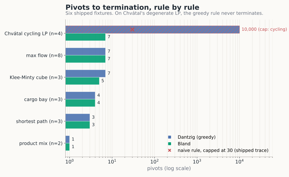
Greedy cycles too, tie-break and all, spinning until the 10,000-pivot cap trips. (The golden trace stops at 30 to keep the committed artifact small; the measurement raises the cap to 10,000 and the cycle still never exits.) So the tie-break I trusted turned out to be just hygiene. With a greedy entering rule, no leaving-row tie-break alone prevents cycling on this program. Only Bland’s rule, which constrains both choices, terminates, in 7 pivots.
The second failure is slowness, and it is the one Klee and Minty made famous in 1972: a family of squashed hypercubes shaped so the greedy rule visits every single corner. The site draws the three-dimensional cube and its 8-stop tour. For this post I generated the family up to dimension 12 and let both rules loose:
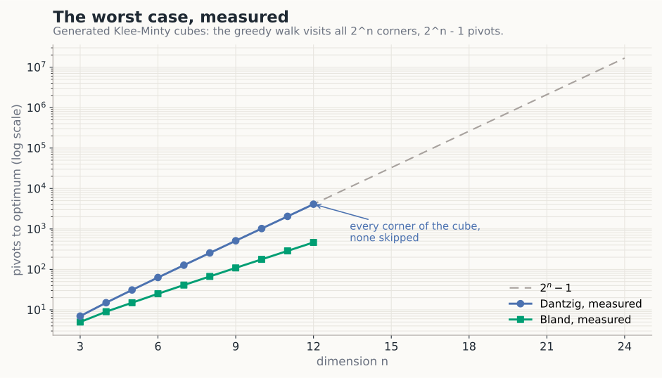
The greedy counts are not approximately exponential, they are exactly $2^n - 1$, every corner of every cube, through all 4,095 pivots of the twelve-dimensional case. Bland takes 465 pivots at n = 12 against those 4,095, though that says nothing general in its favor. Adversarial families exist for Bland too. At n = 200 the corner count is a 61-digit number, which is the site’s way of showing you cannot get there by listing corners. Simplex stays fast in practice because real programs are not adversarial.
The price row
The walk finishes on the top of that staircase, 22: the first corner whose neighbors all sit lower, so no pivot climbs higher and the search stops, exactly the stopping rule the climb started from. By then the solver has computed more than the best plan. The objective row is also holding prices, and the sketch shows what they mean before any algebra:
The cargo problem’s tableau does the same accounting in higher dimension. When its walk finishes, the slack columns of the objective row hold the dual prices: at a non-degenerate optimum, and within the range where the optimal basis keeps holding, that is what one more unit of each limit would be worth. If you know these as Lagrange multipliers, that is exactly what they are: the shadow price on a constraint is the multiplier on it, the sensitivity of the optimum to loosening that limit. It is the same object that turns up in any KKT condition (Boyd and Vandenberghe work out the LP case in chapter 5 of Convex Optimization), and the same reason an SVM keeps only a handful of support vectors. A training point with a zero dual multiplier sits off the margin and moves the boundary not at all, exactly as a slack constraint here carries a zero price and can loosen without changing the plan; the points that set the boundary are the ones whose multiplier is nonzero, the binding constraints.
Three of the cargo problem’s five limits bind at the optimum, so three slack columns of the final z-row carry a nonzero price: $-1/7$ on $x_1 + 4x_2 \le 45$, $-3/7$ on $2x_1 + x_2 \le 27$, and $-1$ on $x_3 \le 4$ (the row stores the objective negated, so flip the signs to read the prices; the explainer renders them as exact fractions instead of $-0.142857$, $-0.428571$, and $-1$). Charge each price against its limit and they stack to exactly the optimal profit: $\tfrac{1}{7}(45) + \tfrac{3}{7}(27) + 1(4) = \tfrac{45}{7} + \tfrac{81}{7} + 4 = 22$. That identity is strong duality.
Full disclosure about those tidy fractions: the solvers compute in ordinary 64-bit floats with an epsilon of 1e-9, in both languages. The fractions are a display-layer reconstruction, snapping a float to the nearest small-denominator rational when one sits within tolerance, and falling back to decimals when none does. Exact rational arithmetic in the engine was never needed at this problem scale, and floats are what keep 64-dimensional fuzz problems cheap. The golden tests would catch any float drift in CI first.
Timing the Rust port
Porting bought trust and deployability. It also set up an unusually clean benchmark, since both engines execute the identical sequence of pivots on the identical arithmetic, and the tests prove the walks identical, so whatever gap the clock shows comes from the execution substrate alone. I timed seeded random dense programs from 4 to 512 variables, five programs per size, medians over repeated runs (nine at the small sizes, tapering to three at the largest, where a single pure-Python solve takes seconds). The harness asserts status, objective, and iteration-count parity between backends on every problem before recording a number.
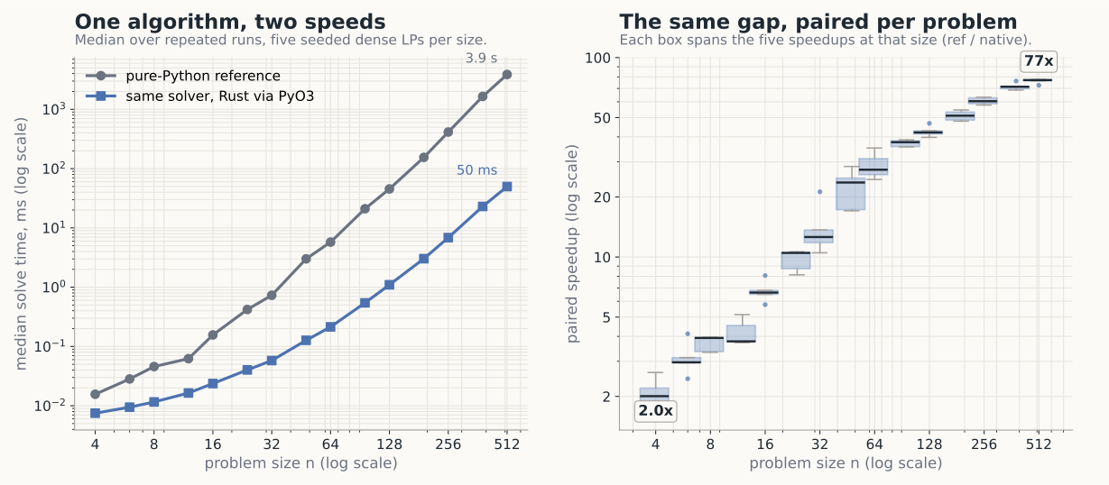
At n = 4 the native engine wins by 2.0x, most of which is Python’s per-call machinery on both sides of a sub-microsecond computation. The gap widens with size. The paired median is 6.6x at n = 16 and 27x at n = 64, and by n = 512 it reaches 77x: the median solve there takes 3.9 seconds in pure Python and 50 milliseconds in Rust for the identical walk (paired medians, so the ratio differs slightly from dividing those two numbers). The boxes in the right panel stay narrow all the way up. Whatever problem the generator draws, the substrate gap comes out about the same. On the shipped fixtures, which are tiny, the gap is a mundane 1.3x to 4.2x, because the PyO3 boundary crossing is a fixed tax on a microsecond-scale job. For the explainer even the slow line would have been fast enough; a drag re-solve is a three-variable problem. The port’s real payoff is elsewhere: the same 714 lines run in the reader’s browser tab and behind the Python API, both under the same tested guarantees.