Diffusion models - building an image generator from scratch, then the ladder to DALL·E 2

Every digit in the sample grid further down this post started as pure static. No digit was retrieved, copied, or stitched together from training images. A small neural network looked at random noise and, step by step, removed its way to a handwritten number. You can replicate the full exercise locally, the whole thing is about three hundred lines of PyTorch.

A diffusion model is a generative model that learns to reverse a gradual noising process. You take real data, destroy it by adding noise in small steps until nothing is left, and train a network to undo one step of that destruction. To generate something new, you hand the network pure noise and let it walk the destruction backwards. That is the entire idea, and as of May 2022 it produces the best image samples the field has: a year ago diffusion overtook the strongest GANs on ImageNet (Dhariwal and Nichol), and every leading text-to-image system now builds on it.

I am writing this the week DALL·E 2 dropped, three weeks after OpenAI first showed it off. You write a caption like “Picard riding on Voyager, through Delta Quadrant’s unique planets” and the model paints it, and right now nobody quite knows how the next year of this goes. Underneath those headline results sits the same denoising loop I am about to build on MNIST, so I want to write it down from inside this specific moment, before the field settles. The post has two parts:

• First I build a denoising diffusion model from scratch and watch it hallucinate digits and clothing
• Then I walk the short, fast ladder of papers, all published between 2020 and last month, that carried this idea from “interesting on CIFAR” to DALL·E 2.

The companion code is at ddpm-from-scratch. Every figure below comes out of it.

The whole idea in one picture

There are two processes here, and they run in opposite directions: one is a fixed noising schedule with no learned parameters at all, and the other is a learned denoiser trained to walk that schedule backwards a single step at a time.

The forward process takes a clean image and adds a small amount of Gaussian noise, then adds a little more, and a little more, for $T$ steps, until the image is indistinguishable from static. This process has nothing to learn. The schedule of how much noise to add at each step is fixed before training starts, with no learned parameters; only the noise itself is drawn fresh at random.

The reverse process is a neural network. It learns to look at a noisy image and undo one step of the forward process, nudging it back toward something slightly cleaner, and stacking a thousand of those small nudges is what walks us all the way from pure static back to a plausible image.

Here is the trick that makes it trainable on a laptop. We don’t have to run the forward process one step at a time during training, because each step only adds Gaussian noise and Gaussians stack into Gaussians, which means we can skip the entire grind and jump straight to the noise level at any step t in a single shot.

Step 1: destroy an image by design

Let the noise schedule be a sequence of small numbers $\beta_1, \dots, \beta_T$ (I used $T = 1000$). Define $\alpha_t = 1 - \beta_t$, and let $\bar{\alpha}_t$ be the running product of every $\alpha$ up to step t:

Then the noised image at step t, given the clean image $x_0$, has a closed form:

Visualize it as a slider, i.e. $\bar{\alpha}_t$ starts near 1 and decays toward 0 as t grows, so early on you keep most of the image and add a whisper of noise, and late on you keep almost none of the image and it is nearly all noise. There is no network in this equation. It is arithmetic, and it is the whole destruction jumped to in one step; the reverse network’s only job, later, will be to walk this line backwards. In code it is two lines:

def q_sample(self, x0, t, noise):

    # jump straight to the noise level at step t ( reparameterization )

    A = extract(self.sqrt_alphas_cumprod, t, x0.shape) * x0
    B = extract(self.sqrt_one_minus_alphas_cumprod, t, x0.shape) * noise

    return ( A + B )

Here is a real 3 from MNIST, run through q_sample at a ladder of increasing t values. Watch it dissolve. Each frame adds a little more noise than the one before it.

That schedule deserves a second look, because the first thing the field improved after the original model was exactly this curve. The original DDPM paper used a linear schedule, where $\beta_t$ grows linearly. A year later, Improved DDPM pointed out that on small images the linear schedule destroys the picture too fast, so the last few hundred steps are nearly pure noise and teach the network almost nothing. Their cosine schedule keeps signal around for longer. I use the cosine schedule, and you can see why below.

Step 2: train a network to undo one step

Now the only learned part. We want a network that, given a noisy image $x_t$ and the step t, removes noise. It could predict either the clean image or the noise that was added; DDPM predicts the noise. So $\epsilon_\theta(x_t, t)$ guesses the $\epsilon$, and the loss is the mean squared error between the true noise and the guess.

This simple form drops out of a variational bound on the data likelihood; the DDPM paper has the derivation. The training step is short:

def p_losses(self, model, x0, t):
    noise = torch.randn_like(x0)            # the target
    x_t = self.q_sample(x0, t, noise)       # noise the image to level t
    predicted = model(x_t, t)               # ask the network to guess the noise
    return F.mse_loss(predicted, noise)     # how wrong was it

The full training loop is the loop you already know from any supervised model, with one extra line that picks a random noise level per image:

for x0, _ in dataloader:
    t = torch.randint(0, T, (x0.size(0),))   # a different noise level per image
    loss = diffusion.p_losses(model, x0, t)
    opt.zero_grad(); loss.backward(); opt.step()
    ema.update(model)                        # keep a moving average of the weights

The ema.update line earns its keep. Sampling from an exponential moving average of the weights rather than the live weights noticeably cleans up the samples in my runs, and it costs nothing but a copy of the parameters.

What about the network itself?

It is a U-Net, with one diffusion-specific addition: the step t becomes a sinusoidal embedding injected into every block, so one set of weights can behave differently at high noise and low noise. The figure below carries the shape. Mine is about 10M parameters, small by any standard, and we won’t walk through it line by line; the whole thing is in unet.py

Trained on MNIST for forty epochs, the loss falls fast and then crawls, and the crawl is fine, because diffusion loss values are a poor proxy for sample quality and the grids keep sharpening for a long time after the number itself has stopped moving.

Step 3: sample by denoising pure noise

Training taught the network to undo one step. Sampling chains it. Start from pure Gaussian noise $x_T$, ask the network for the noise, form a slightly cleaner mean by subtracting it, add back fresh randomness scaled by the step’s variance, and step down to $x_{t-1}$. (That variance is fixed by the schedule here; Improved DDPM later made it learnable, which is the log_var term in the code below.) That last bit of randomness is what keeps each run different; drop it and the reverse process turns deterministic, which is exactly the trick DDIM turns into a feature later. The reverse step in code, where the subtraction lives inside p_mean_variance:

@torch.no_grad()
def p_sample(self, model, x_t, t):
    mean, log_var, _ = self.p_mean_variance(model, x_t, t)  # uses eps_theta
    noise = torch.randn_like(x_t)
    nonzero = (t != 0).float().reshape(-1, 1, 1, 1)          # no noise on the last step
    return mean + nonzero * (0.5 * log_var).exp() * noise

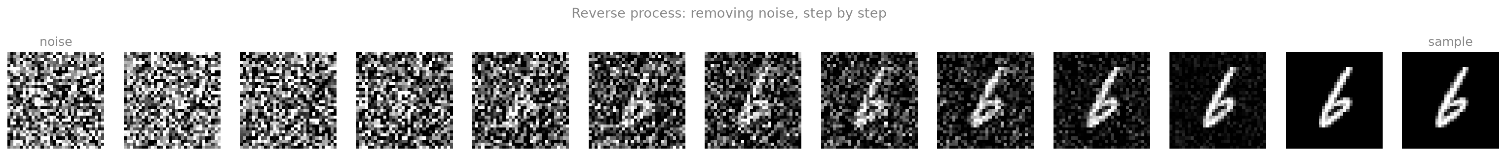
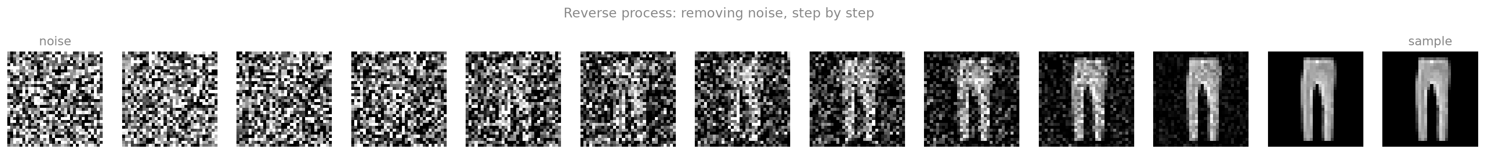
Run that from t = 999 down to t = 0. An image condenses out of the static. This is the figure that made diffusion click for me: a single sample, photographed every hundred steps as it resolves from noise into a legible handwritten digit.

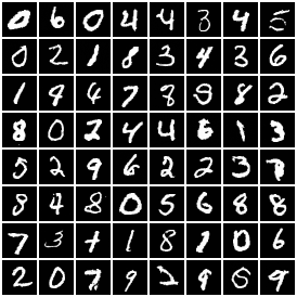
Now scale it up. Do this for sixty-four independent noise seeds and you get a whole sheet of digits, not one of which exists anywhere in the MNIST training set.

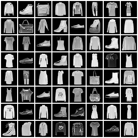
Retraining on clothes

I didn’t believe the MNIST grid. Ten digit shapes is exactly the kind of thing a small network can memorize outright, so before trusting any of it I re-ran the identical code on clothes. I changed one command-line flag, --dataset fashion, retrained the same architecture on Fashion-MNIST, and touched nothing else. Same schedule, same loss, same sampler.

Making it usable: DDIM and fewer steps

There is a catch I have been quiet about. Sampling ran the network a full thousand times to produce a single image, which is tolerable for a blog post and ruinous the moment you want more than a handful of them, so the field went looking for a shortcut and found one almost immediately, in DDIM (Song, Meng, and Ermon, late 2020).

DDIM reuses the exact same trained weights with no retraining, and it reinterprets the reverse process so that the steps are no longer required to form a Markov chain, which lets you skip most of them and, in its deterministic ($\eta = 0$) setting, makes the same starting noise always map to the same image every time you run it. The per-step logic is “guess the clean image, then jump partway back toward it” (schematic):

x0  = predict_clean_image(img, t, eps)                   # invert the forward equation
img = sqrt(abar_prev) * x0 + sqrt(1 - abar_prev) * eps   # re-noise to an earlier step

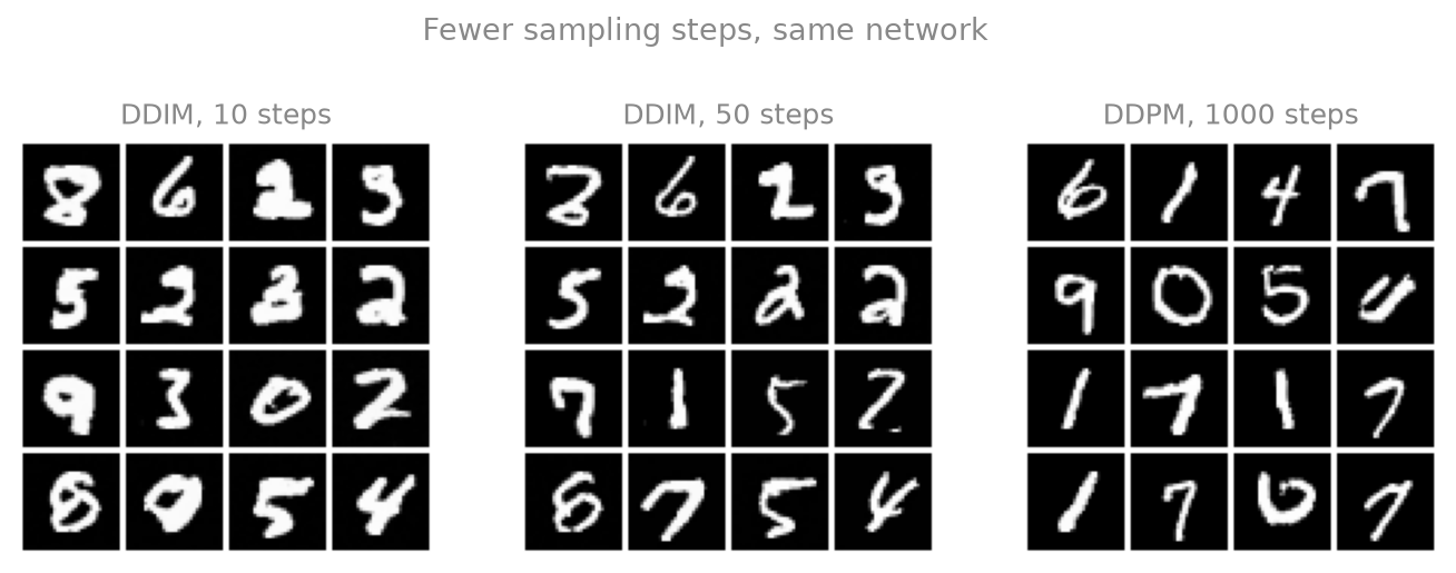
The practical payoff is blunt. I sample in 50 steps instead of 1000, a clean 20x speedup, with barely any loss in quality that the eye can catch. Below, the same network sampled with 10, 50, and 1000 steps.

This is where the from-scratch model points straight at the rest of the field. Sampling is cheap now. The objective is stable. So the next questions almost ask themselves: can we make the samples sharper, can we steer exactly what gets generated, and can we afford to run any of this at megapixel resolution instead of on twenty-eight-pixel digits.

One note before the papers, because the model I built has a gap the next section leans on. It draws a digit, never the digit you ask for, because it never saw a single label during training, and conditioning fixes that with one small change: you hand the network a class label alongside the timestep, folded in as one more embedding exactly like t, and then you train it to denoise with the label held in view. Every kind of steering below is built on that one hook, so I added it to my MNIST model and trained the conditional version, which the guidance section puts to work.

How this became DALL·E 2

Everything above is the 2020 core: DDPM plus DDIM. What turned it into the system that drew the astronaut on the horse is a short ladder of papers, each fixing one specific limitation. Here is that ladder, in order.

Only one rung below, classifier-free guidance, is one I run myself on MNIST. If you want the hands-on part, skip straight to it; the rest is context for how the same denoising loop scaled up to DALL·E 2.

Three of these rungs need no new experiments here - two are already folded into the build above, and one is a change of notation. DDIM is where a thousand sampling steps became fifty, which is what made everything downstream cheap enough to iterate on. Improved DDPM (Nichol and Dhariwal, 2021) gave me two things at once: the cosine schedule I used, and the trick of letting the network learn the reverse-step variance instead of fixing it. One function, better everything after. Score matching (Song and Ermon, 2019) is stranger. It looked like a separate idea until Song and colleagues showed in late 2020 that it is diffusion wearing different notation: predicting the noise is, up to a time-dependent scaling, the same as estimating the gradient of the data density, and both fall out of one continuous-time stochastic differential equation. So the words are interchangeable. When a paper says “score-based,” read “diffusion.”

Beating GANs: classifier guidance (May 2021). Dhariwal and Nichol tuned the architecture and added classifier guidance: at sampling time, nudge each step with the gradient of a classifier trained on noised images toward the class you want. The result beat the best GANs on ImageNet, which is the moment the field’s default quietly flipped from GANs over to diffusion, though the catch in the title is real and worth stating plainly: this was one benchmark, ImageNet, measured on one carefully tuned setup. What guidance actually buys is a knob that trades sample diversity for fidelity, by sharpening the conditional distribution.

Dropping the classifier: classifier-free guidance (Dec 2021). Training a separate classifier on noisy images is awkward, and it pins you to a fixed set of labels, which is useless for free-form text. Ho and Salimans (NeurIPS 2021 workshop) removed it. Train one network that sometimes sees the condition and sometimes sees a blank, then at sampling time extrapolate between the two predictions:

Here $c$ is the condition (a class, a caption), $\varnothing$ is the blank, and $w$ turns the steering up. Read it as extrapolation: the blank prediction is the way the network would denoise with no caption, the gap to the conditioned prediction is the caption’s contribution, and $w$ pushes the noise estimate further along that gap. Most implementations write the same thing with a guidance scale $s = 1 + w$, where $w = 0$ (so $s = 1$) means no steering, so if you compare two codebases and the numbers look off by one, that is why. Classifier-free guidance is the workhorse of every strong text-to-image model that followed.

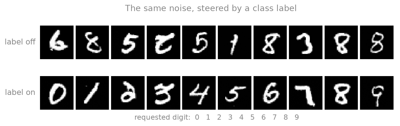
This is the one rung I can run myself. Classifier-free guidance needs a model that can sample both with and without the label, so I trained exactly that on MNIST: a conditional U-Net with the label dropped 15% of the time. First the basic question, does the label even steer it? Same ten starting seeds, run once ignoring the label and once told which digit to draw:

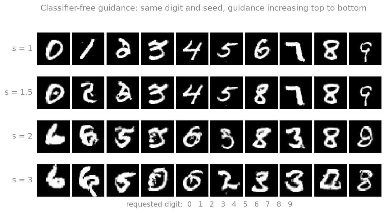
Now turn the guidance dial up. More guidance trades diversity for fidelity, sharpening each sample toward its class. On a model this small, the usable range is narrow:

The last two rungs turned that steering into pictures from captions. Diffusing directly on megapixel pixels is brutally expensive, since the U-Net runs at full resolution a thousand times over, so latent diffusion (Rombach and colleagues) moved the whole process into the compact latent space of a pretrained autoencoder, cut the cost by roughly an order of magnitude, and wired in cross-attention so you can condition on text or layout. That is the architecture that would become Stable Diffusion later in 2022. As I write this, it does not exist yet. GLIDE had already shown classifier-free guidance beats CLIP-based guidance for following captions. Then DALL·E 2, three weeks ago, restructured everything around CLIP: a prior (itself a diffusion model) turns the caption into a CLIP image embedding, and a diffusion decoder turns that embedding into a picture, so there is diffusion on both ends with classifier-free guidance doing the steering. The authors call it unCLIP, a different lineage from latent diffusion.

What is still hard

A few things that were still genuinely unsolved, from where I sat in May 2022.

Sampling is still slow. A GAN generates in a single forward pass; DDIM helped a lot, fifty steps instead of a thousand, but that is still fifty forward passes to the GAN’s one, and the race to cut that further has already started: progressive distillation, out this February, halves the step count and then halves it again. Evaluation is shaky too. FID (Fréchet Inception Distance) is the standard number and it is a blunt instrument, and “does this image match the caption” has no clean metric at all.

The compute gap is the core one. My model is about 10M parameters trained for forty epochs on a laptop, and the results that make headlines come from networks orders of magnitude larger fed far more data, so that difference in scale is most of what separates “can build this on MNIST” from “can build DALL·E 2.”

Guidance is not free either. The figure above showed its cost in miniature: the lower rows thicken, oversaturate, and slide off the manifold of real images.

Build it yourself

The model in this post is small. Small enough to read in one sitting and train on a laptop, which was the whole point of building it this way. If you want the denoising idea to stop being abstract, clone the repo, run train.py, and watch the sample grid fill in epoch by epoch, keeping in mind that the forward process, the loss, and both samplers are each only a handful of lines, exactly as shown above. Nothing here is hidden.

Browse the code Read the DALL·E 2 paper More deep learning from scratch