Singular value decomposition - rebuilding an image from its largest stretches

The singular value decomposition is the statement that every matrix, whatever is in its entries, moves space in three steps : a rotation, a stretch along perpendicular axes, and a second rotation. Any real matrix factors as :

where $U$ and $V$ are orthogonal (their columns are perpendicular unit vectors, so they rotate without distorting anything) and $\Sigma$ is diagonal and nonnegative. The diagonal entries of $\Sigma$, sorted so that $\sigma_1 \ge \sigma_2 \ge \dots \ge 0$, are the singular values : the stretch factors, ranked by how much they matter.

That one sentence is enough to rebuild a galaxy from a sliver of its data. A 512 by 512 photograph of the Whirlpool galaxy is, to numpy, a matrix of 262,144 numbers. Keep its fifteen largest stretches and you are storing 15,375 numbers, under 6% of the original, and the spiral arms are already unmistakably visible. A theorem from 1936 guarantees that nothing else of that size does better, and tells you the error before you compute a single pixel.

In this post, we work with two objects - a 2x2 matrix that we can watch move the plane, and one photograph. We explain two concepts, PCA and least squares, each with a short section. The one thing I deliberately skip is how a cpu actually finds singular values.

One matrix, one circle

A 2x2 matrix :

Columns tell you where the two basis vectors land, but not what $A$ does to space as a whole, so the better probe is to feed it every direction at once : all the unit vectors, the whole unit circle, watched together as they pass through.

An ellipse, tilted and three times longer in one direction than the other. The only freedoms it has are which perpendicular axes to use, how hard to stretch along each, and where to point the result.

The ellipse axes have names

Label the long semi-axis of the ellipse $\sigma_1 u_1$ : its length is $\sigma_1$, the largest stretch, and the unit vector $u_1$ is the direction it points. The short semi-axis is $\sigma_2 u_2$, perpendicular to the first. Then walk backwards : somewhere on the input circle sits the unit vector that $A$ sent to the tip of the long axis; call it $v_1$, and call the preimage of the short axis tip $v_2$.

There is a second way to arrive at $v_1$ : over all unit vectors $v$, which one does $A$ stretch the most? That is $v_1$, the achieved length $\lVert A v_1 \rVert$ is $\sigma_1$, and restricting to directions perpendicular to $v_1$ and asking again gives $v_2$. The line through $v_1$ is the best-fit line through a cloud of points in n-dimensions (the rows of $A$), the plane through $v_1, v_2$ is the best-fit plane.

Rotate, stretch, rotate

$V$ contains $v_1, v_2$ in its columns, $U$ contains $u_1, u_2$, and $\Sigma$ contains the two stretch factors. The equation $A = U \Sigma V^{\mathsf{T}}$ then reads, right to left, as a recipe applied to any input :

First $V^{\mathsf{T}}$ rotates the plane so that $v_1$ and $v_2$ lie along the coordinate axes, and $\Sigma$ then stretches by 3x and 1x, independently. Then $U$ rotates the stretched result into its final orientation. All the shearing, tilting messiness that $A$ seemed to have was an artifact of looking at it in the wrong coordinates; in the right input frame and the right output frame, every matrix is diagonal.

using numpy :

import numpy as np

A = np.array([[2.1907, 1.4836],
              [0.4483, 1.6731]])

U, S, Vt = np.linalg.svd(A)
print(S)

[3.0000682  1.00003136]

Not exactly 3 and 1, because we rounded the entries of $A$ to four decimals when writing them down, and the singular values report the damage in the fifth digit. That is because this matrix was synthetic : I built it as a 45 degree rotation, then a stretch by $\mathrm{diag}(3, 1)$, then a 30 degree rotation, and the printed entries are that final output. The decomposition recovered the recipe from the entries alone.

Two conventions hide in that call :

• numpy returns back Vt, the transpose of $V$, not $V$ itself
• with full_matrices=False (used below) it returns the thin form that skips the parts multiplied by nothing ( numpy docs )

Dropping the smaller stretch

The matrix-of-rotations picture has an equivalent that turns out to be the useful one for data. Multiply the factorization - cell by cell and it becomes a sum:

Each term is an outer product, a column pattern $u_i$ x a row recipe $v_i^{\mathsf{T}}$ weighted by $\sigma_i$, and I think of each one as a block. A block is the simplest matrix there is, rank one, every row a multiple of every other, and it costs only $m + n + 1$ numbers to describe no matter how large the matrix is. SVD rewrites your matrix as a sum of blocks, sorted by weight.

Sorted by weight implies a natural potential cut : keep the heavy blocks and drop the light ones.

Numerically the heavy block of our matrix is :

and comparing it against $A$ entry by entry, the worst miss is 0.61, which is exactly the largest entry of the discarded $\sigma_2 u_2 v_2^{\mathsf{T}}$. For a 2 by 2 matrix this trade is silly : the block costs five numbers to store where the matrix cost four. This turns more interesting when the matrix is large and its stretches are unequal, as is the case in most real-world datasets.

The matrix is a galaxy

I pulled a 512x512 cutout of M51, the Whirlpool galaxy, from the SDSS DR17 SkyServer cutout service, centered on RA 202.4842, Dec 47.2306 at 1.4 arcseconds per pixel, wide enough to catch both the spiral and its companion NGC 5195. The exact request URL sits at the end of the post, so every number below can be re-run against the same frame. Collapsed to grayscale luminance it is one matrix, 512 rows by 512 columns, 262,144 numbers between 0 and 1.

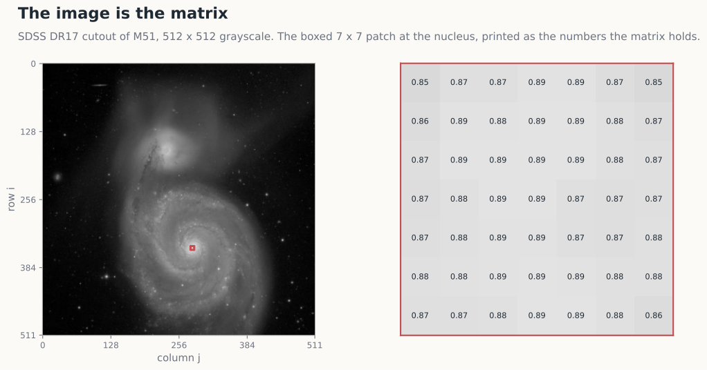
from skimage import io, color

A = color.rgb2gray(io.imread("m51_sdss_512.jpg"))   # 512 x 512, values in [0, 1]
U, s, Vt = np.linalg.svd(A, full_matrices=False)     # s has 512 entries

Our initial 2x2 matrix had two singular values, this one has 512 :

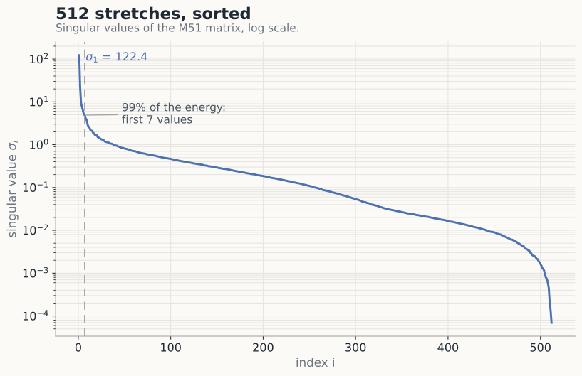
The top value, $\sigma_1 = 122.4$, towers over $\sigma_2 = 21.8$ by a factor of 5.6, and the tail decays over six orders of magnitude. The physical reading : about half the frame is black given a small margin, and most of what is not black is smooth, the broad glow of two galaxy disks. Smooth large-scale structure is exactly what a few blocks reproduce well; the pinpoint stars scattered across the frame are another matter though.

Square the singular values and you get the “energy” most textbooks use : $\sigma_1$ alone carries 94.6% of this image’s “energy”, and the first seven values carry 99%. By that measure - seven blocks should nearly suffice, and yet at $k = 7$ the frame is still smudges. Squaring inflates the lead of the front-runner, so energy fractions crowd toward 100% long before pictures look like anything meaningful. The yardstick that tracks what the eye sees is the relative error $\lVert A - A_k \rVert_F / \lVert A \rVert_F$, which at $k = 7$ still stands at 9.7%.

block by block

The rank-$k$ reconstruction keeps the $k$ heaviest blocks :

def rebuild(k):
    return (U[:, :k] * s[:k]) @ Vt[:k, :]

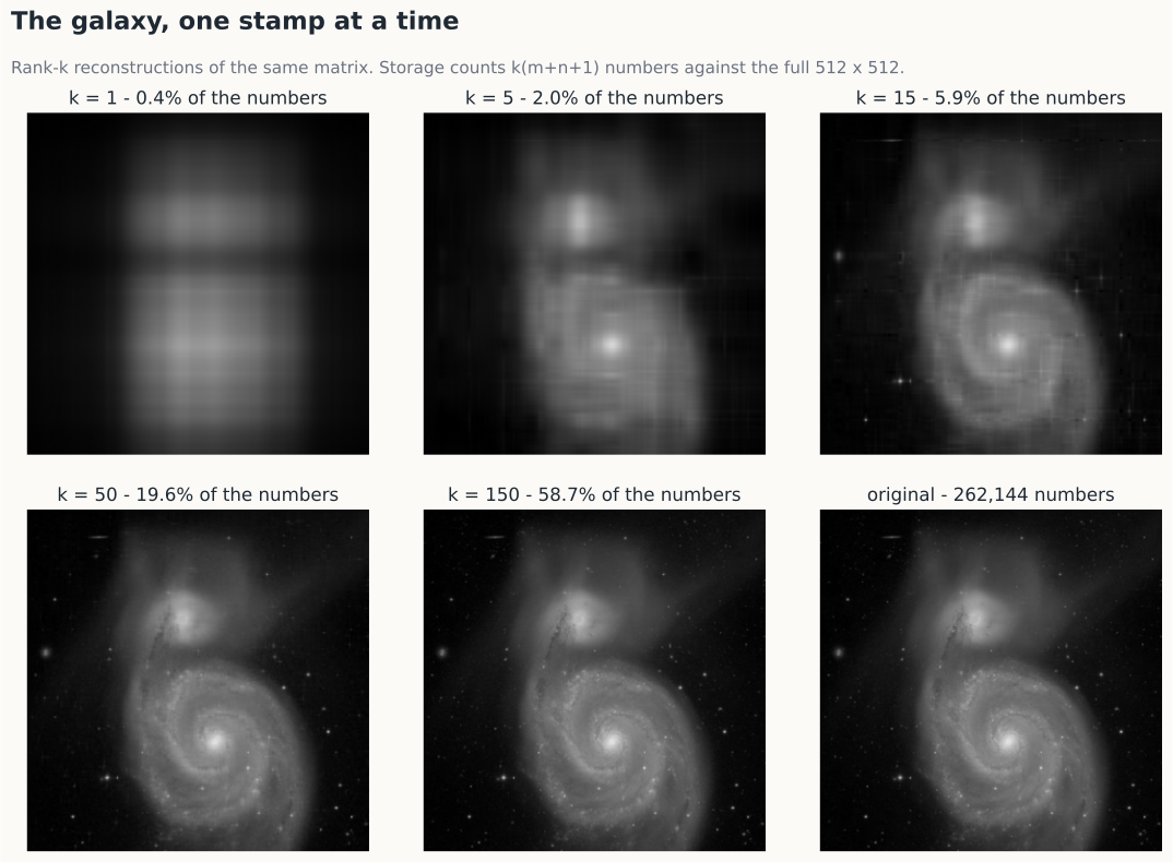
Each block is a single column pattern times a single row recipe, so $k = 1$ can only paint axis-aligned bands. First panel is a bright horizontal belt across the rows where the galaxies live, crossed by a vertical one over the columns that hold them. By $k = 5$ the two disks exist as blobs. At $k = 15$, costing 5.9% of the numbers, the spiral arms are unmistakable, though every miss still smears into horizontal and vertical streaks, the outer-product basis showing through. At $k = 50$ the streaks are gone, and from $k = 150$ eyes cannot tell the reconstruction from the original at this size, with 1.6% relative error.

Compare the $k = 15$ panel against the original and one class of objects is conspicuously late : the foreground stars. A star is two or three bright pixels, which contributes almost nothing to the Frobenius energy the approximation is optimizing, so the top blocks spend their budget on the broad disks and leave the stars for the deep tail. The glow is cheap; the stars are expensive. If your science lives in point sources, truncated SVD is a lossy filter aimed directly at the thing you care about, which is worth knowing before you use it to denoise anything.

One caveat before anyone tries this on a photo library : this is not how images are compressed in practice. JPEG runs a fixed cosine transform on local 8x8 blocks; it has no 512-number global patterns to fit and nothing to solve, and at these quality levels it is far cheaper. The rank-$k$ ledger here, 0.4% at $k = 1$ to 58.7% at $k = 150$, is the pedagogical price sheet for a global, image-specific basis.

As good as rank k gets

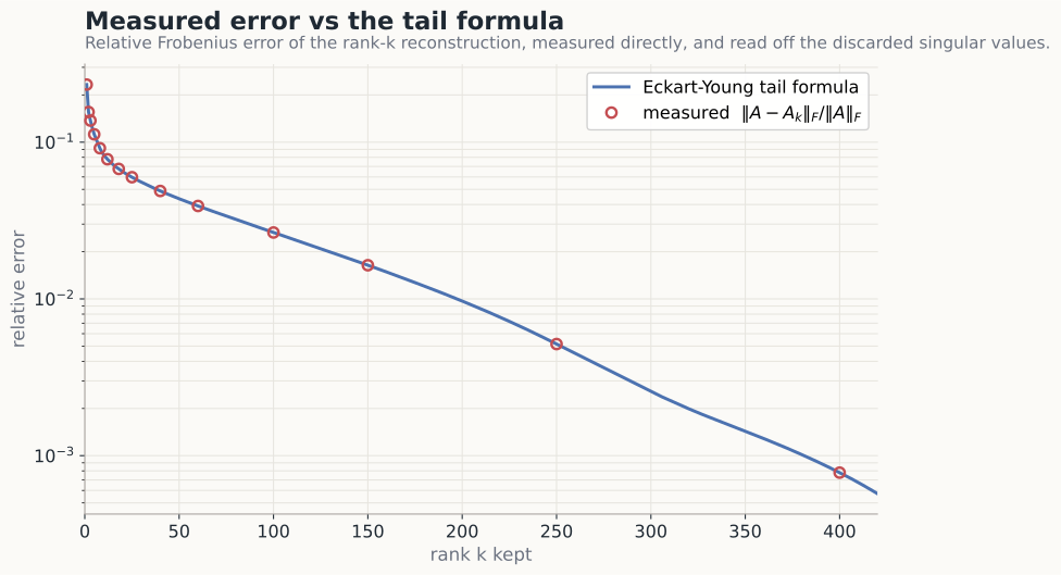
The guarantee is the Eckart-Young theorem, published in 1936 and extended by Mirsky in 1960. Among all matrices of rank at most $k$, with no restriction to SVD-shaped candidates, the truncated sum $A_k = \sum_{i \le k} \sigma_i u_i v_i^{\mathsf{T}}$ is the closest to $A$, in the Frobenius norm, in the spectral norm, and, after Mirsky, in every norm that is indifferent to rotations.

The discarded weights are the error, so the spectrum in the second figure was already a complete error catalog for every possible truncation, available before reconstructing anything. It can be checked in two lines:

k = 15
measured  = np.linalg.norm(A - rebuild(k)) / np.linalg.norm(A)
predicted = np.sqrt(np.sum(s[k:] ** 2)) / np.linalg.norm(A)

The same picture in PCA

PCA ~ mean centered + truncated SVD output

Take $n$ data points in $d$ dimensions, subtract the column means, and call the centered matrix $X$. Principal component analysis asks for the directions along which the cloud varies most, subject to being mutually perpendicular, which is verbatim the greedy question from earlier asked of $X$. The answers are its right singular vectors : the first principal direction is $v_1$, the second is $v_2$, and the variance captured along $v_i$ is $\frac{\sigma_i^2}{(n - 1)}$.

The Gram matrix makes the link mechanical : $X^{\mathsf{T}} X = V \Sigma^2 V^{\mathsf{T}}$, so the eigenvectors of $X^{\mathsf{T}} X$ are the right singular vectors, its eigenvalues are the squared singular values, and dividing by $(n-1)$ turns it into the covariance matrix carrying exactly the variances above. This is also why we usually compute PCA through an SVD of $X$ rather than by forming $X^{\mathsf{T}} X$ : squaring the matrix squares its condition number, and the small components drown first. “keeping the components before the elbow” from an analysis of principal components is the same as keeping fifteen blocks of a galaxy here.

Running the film backwards

What do you do with $Ax = b$ when it has no solution, the everyday situation of more equations than unknowns? Strang’s answer in 18.06 is to project $b$ onto the column space of $A$ and solve for the projection, which is what least squares is.

The SVD version is the three-moves picture run in reverse : $A$ rotated by $V^{\mathsf{T}}$, stretched by $\Sigma$, and rotated by $U$, so undo each move last-first, rotating back by $U^{\mathsf{T}}$, dividing by every stretch you can divide by, rotating back by $V$. The only move that can refuse to reverse is the stretch, where a $\sigma_i = 0$ flattened a whole direction to nothing, and there division is impossible; the convention is to leave those directions at zero rather than invent information the matrix destroyed. The result is the pseudoinverse

with $\Sigma^{+}$ holding $1/\sigma_i$ for each nonzero stretch and 0 elsewhere. The vector $x = A^{+} b$ is the least-squares solution, and when even that is not unique, it is the shortest one. This is what np.linalg.lstsq and np.linalg.pinv compute underneath, and it is why they keep working on the degenerate systems that make the textbook normal equations fall over.

In the meantime, the cutout service takes any coordinates you like : pick your own galaxy, pull its 512 stretches, and count how few of them matter.

Sources

• Gregory Gundersen, Singular Value Decomposition as Simply as Possible, 2018. The geometric build-up, with the barn-shear intuition.
• John Hopcroft and Ravindran Kannan, Computer Science Theory for the Information Age, chapter 4. The greedy best-fit-subspace development and both optimality proofs.
• Gilbert Strang, MIT 18.06, Least Squares unit, OCW 2011. Projection, normal equations, pseudoinverse.
• G. W. Stewart, On the Early History of the Singular Value Decomposition, SIAM Review, 1993.
• Carl Eckart and Gale Young, The Approximation of One Matrix by Another of Lower Rank, Psychometrika 1(3), 1936.
• Lloyd Trefethen and David Bau, Numerical Linear Algebra, SIAM 1997, Lecture 4. The hyperellipse picture.