Clinical evaluation
What a clinic would actually need
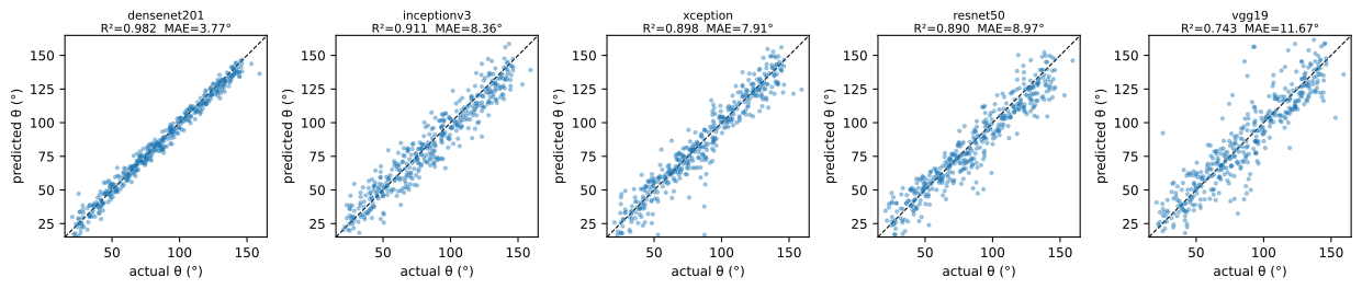
A clinic does not act on a single number. It acts on a number with a band around it, an honest account of how far it sits from the reference it would replace, and some assurance that the model is reading the anatomy rather than an artefact. This page reports four such checks on the tuned DenseNet201, all recomputed from the saved patient-level out-of-fold predictions.
These results are a research-grade characterisation, not a deployment claim. They are computed on the same small single-center cohort — roughly ten volunteers, 84 base images, one Sonix OP scanner, common carotid artery only — and against a single MATLAB-GUI reference reading per image. Read them as evidence about the estimator’s behaviour, not as a clearance for clinical use.
A band, not just a number
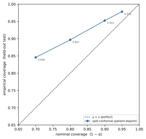
A point estimate of the insonation angle is only useful if its uncertainty is legible. We wrap the tuned DenseNet201 in a split-conformal procedure: hold out a calibration set, take the empirical quantile of the absolute residuals, and emit a symmetric prediction interval whose half-width is that quantile. For a target miscoverage \(\alpha\) and calibration residuals \(r_i = \lvert \theta_{\text{true},i} - \theta_{\text{pred},i}\rvert\), the half-width is
\[q_{1-\alpha} = \operatorname{Quantile}_{1-\alpha}\big(\{r_i\}\big), \qquad \text{interval} = \big[\,\hat{\theta} - q_{1-\alpha},\; \hat{\theta} + q_{1-\alpha}\,\big].\]The split is patient-disjoint (a group-conformal split: 900 calibration rows and 1200 test rows, with no patient appearing in both), so the interval is distribution-free and finite-sample valid. At a single seed-42 split the empirical coverage meets or exceeds the nominal level at every band, which is why the intervals are wide but honest.
| Nominal level | Interval half-width | Empirical coverage |
|---|---|---|
| 80% | ±15.01° | 89.7% |
| 90% | ±20.50° | 95.2% |
| 95% | ±26.03° | 97.8% |
The headline band is ±20.50° at the 90% level, with empirical coverage of 95.2% — at or above nominal. The interval is honest precisely because it is wide: roughly forty degrees of total width is the price of distribution-free validity on a cohort this size.
The conformal split sits on top of pooled out-of-fold predictions, which can make the bands look mildly optimistic.
The OOF predictions on which these intervals are calibrated were produced across the cross-validation folds rather than on a single fully held-out test set, and the same pooled-OOF predictions feed the stacked ensemble reported on the Results page. Stacking and calibrating on out-of-fold predictions can be mildly optimistic, so treat the empirical coverage as an estimate from a single seed-42 patient-disjoint split (900 calibration rows, 1200 test rows), not a guarantee.Figure 1
Agreement, not inter-observer
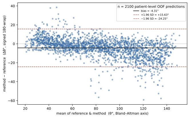
The estimator would, in practice, stand in for a sonographer’s manual angle setting, so the right question is how far it sits from the reference reading it would replace. A Bland–Altman analysis plots the signed difference against the mean of the two readings. Per sample, across all 2,100 views, the bias is −4.31°, with 95% limits of agreement of −24.25° … +15.63° (n=2,100). Aggregated per patient, the bias is −4.56°, with limits of agreement of −16.87° … +7.75° (n=12). The bias is small and negative: the model reads slightly lower than the reference.
This is a method-vs-reference comparison against a single reading, not an inter-observer agreement study.
There is exactly one MATLAB-GUI reference reading (theta_true) per image, so the Bland–Altman analysis measures how the model agrees with that single reference — not how two independent readers agree with each other. The reference is itself a noisy estimate of the true angle, and we cannot separate model error from reference error. The differences are also signed with a 180°-periodic wrap, and the per-sample n=2,100 counts 25 coupled rotation copies of each of the 84 base images, not 2,100 independent measurements.
Figure 2
De-rotation cuts the per-image error by about two-fifths
The augmentation that builds the training corpus is also a tool at inference. Each of the 84 base images carries 25 rotation views; median rotation test-time augmentation de-rotates every view back to the base frame and reduces them circularly (180°-periodic, seam-safe). On the base images this takes the raw base-image MAE from 7.80° down to 4.72° under the circular median (and to 5.31° under the circular mean) — cutting the per-image error by roughly 40%.
Rotation TTA, base-image MAE
7.80° → 4.72° (circular median over rotations); 7.80° → 5.31° (circular mean). Measured on the 84 de-rotated base images.
The 7.80° base-image figure is on a different footing from the headline patient-level numbers.
The 7.80° → 4.72° reduction is measured on the 84 de-rotated base frames, which is not the same population as the patient-level pooled-OOF evaluation. The 7.80° base-image MAE is the like-for-like starting point for this de-rotation experiment, and it should not be read directly against the 5.93° / 8.53% patient-level headline reported on the Results page.It looks at the vessel wall
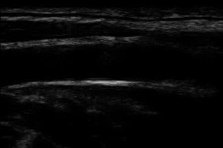
A model that reports an angle should be reading the anatomy that defines the flow axis. Grad-CAM attributions for the tuned DenseNet201 localise on the vessel wall — the longitudinal common-carotid boundary that fixes the orientation — consistent with the network keying on the geometry rather than on an artefact or label leak.
Figure 3
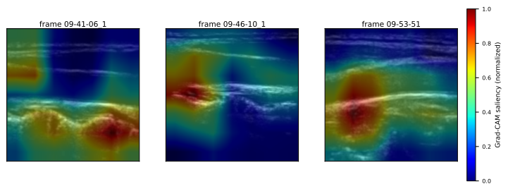
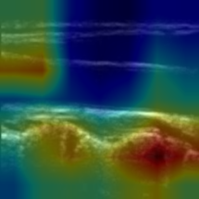
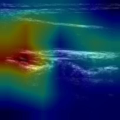
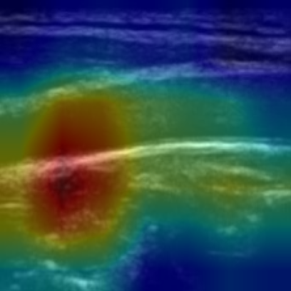
These attributions are illustrative, not a cohort-wide attribution study.
The panels above are three hand-picked frames at the coarse Grad-CAM grid resolution. They are qualitative evidence that the network attends to the vessel wall on these examples; they are not a quantitative, cohort-wide attribution analysis, and they do not certify that the model never relies on an artefact elsewhere.Explore the predictions
The explorer below is driven by the real saved out-of-fold predictions for the tuned DenseNet201 on the study images. Pick one of the 84 base images, scrub the rotation, and read the reference angle, the model’s estimate, the signed residual, and the ±20.50° conformal band on a number line. Nothing here is computed in the browser beyond the signed error \(\theta_{\text{pred}} - \theta_{\text{true}}\); the angles and the band are the precomputed values from the evaluation.
These are precomputed out-of-fold predictions, not live in-browser inference.
The explorer reads precomputed real predictions exported fromresults/predictions/tuned_densenet201_oof.csv — the same pooled-OOF predictions used throughout this page. It is a viewer over saved numbers, not a live model; running the network in the browser on a freshly uploaded image is out of scope for this version.
Figure 4