Method
How the estimator is built, and why each choice is load-bearing
The pipeline is small on purpose. Eighty-four carotid images become a labelled regression corpus by rotation; a frozen ImageNet backbone turns each view into features; a shallow head reads the angle off those features. Every step is a deliberate choice, and one of them — how we pool the spatial feature map — does most of the work.
We report a single estimator under two sampling protocols, and this section walks the pipeline in order: the data and the rotation augmentation that supplies the labels; the two protocols and the distinct question each one answers; the frozen backbone and the orientation-preserving head; the head’s tuning on cached features; and the cross-validated ensemble that gives the best estimator. Throughout, image-level and patient-level numbers are kept explicitly apart, because they measure different things.
The four metrics, defined exactly
Every result on this site is one of four numbers, computed as the codebase computes them. For a set of \(n\) test views with reference angles \(\theta_i\) and predictions \(\hat\theta_i\):
\[\text{MAE} = \frac{1}{n}\sum_{i=1}^{n}\bigl|\hat\theta_i - \theta_i\bigr|, \qquad \text{RMSE} = \sqrt{\frac{1}{n}\sum_{i=1}^{n}\bigl(\hat\theta_i - \theta_i\bigr)^2},\] \[\text{MAPE} = \frac{100}{n}\sum_{i=1}^{n}\frac{\bigl|\hat\theta_i - \theta_i\bigr|}{\bigl|\theta_i\bigr|}, \qquad R^2 = 1 - \frac{\sum_i (\hat\theta_i - \theta_i)^2}{\sum_i (\theta_i - \bar\theta)^2}.\]MAE is the average absolute error in degrees; RMSE penalizes large misses more heavily; MAPE expresses the error relative to the angle, which is the figure most comparable to the EMBC 2019 paper; \(R^2\) is the fraction of angle variance explained. We lead with MAPE and MAE throughout.
Eighty-four images become 2,100 labelled views
The cohort is the one from the original EMBC 2019 study, drawn from the public SPLab (Brno) ultrasound database: 84 B-mode images of the common carotid artery in longitudinal section, from about ten volunteers (mean age 27.5 ± 3.5 years, usually eight images per volunteer). Acquisition used a single Sonix OP scanner, subject supine with the neck rotated, imaging the right common carotid at roughly 390 × 330 pixels. The supervised target is the Doppler angle \(\theta\), the angle between the ultrasound beam and the long axis of the vessel, which enters the Doppler equation through \(\cos\theta\) and is set by hand at the scanner.
The database carries no clinical Doppler-angle annotation, so a reference \(\theta\) was measured offline by one operator in a custom MATLAB interface, drawing a line along the vessel wall and recording its inclination. This single hand-drawn reading is the only ground truth available per image.
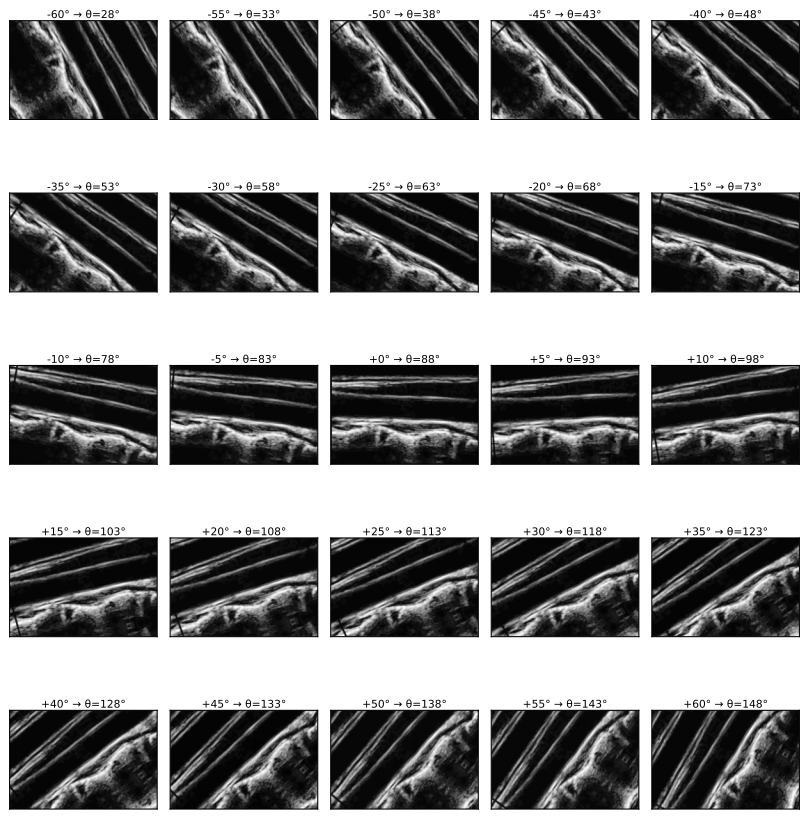
To build a labelled regression corpus, each base image is rotated through a fixed grid spanning [−60°, +60°] in 5° steps, giving 25 oriented views per image and 84 × 25 = 2,100 views in total. The label of a rotated view is the base-image reading plus the applied rotation: the increment is exact, so the network learns to read off relative image orientation. Each view is contrast-equalized with CLAHE before feature extraction, which normalizes the wide dynamic range of B-mode speckle and stabilizes the frozen-backbone features.
The 2,100 views are not 2,100 independent observations.
They are 25 geometrically coupled copies of each of 84 base images, drawn from about ten volunteers, giving a three-level hierarchy — volunteer → base image → rotated view — that the two sampling protocols below treat differently. The label is exact only relative to the single base-image reading, and inherits whatever error that reading carries. The cohort is young, healthy, single-center, and carotid-only, so it supports no conclusions about diseased, aged, or tortuous vessels.
Figure 1
Two protocols, two questions
The same 2,100-view corpus and the same frozen features admit more than one principled train/test partition. We report and tune the estimator under two, each answering a distinct question.
| Protocol | Partition | Question it answers |
|---|---|---|
| Image-level sampling | Random split over the 2,100-view augmented corpus — the original study's protocol | How accurately does the model read \(\theta\) across the full population of orientations the augmentation spans? |
| Patient-level sampling | Whole subjects held out with GroupKFold — no subject's views in both train and test | How well does the model generalize to a previously unseen patient? |
Image-level sampling is the standard way to score a model on an augmented dataset, and it is the regime in which the published headline numbers were reported. Patient-level sampling is the stricter lens: it measures cross-subject generalization, which is harder because the estimator can no longer rely on subject-specific appearance. Holding the model, backbone, head, and training budget fixed and changing only the partition is itself an informative measurement — the gap between the two protocols quantifies how much of the within-population accuracy is anatomy-specific. The patient-level numbers are the clinically relevant ones, and we read them as such.
The patient groups are 12 time-clustered proxies, not verified subject IDs.
The SPLab filenames do not encode volunteer identity, so we recover subject groups by clustering on acquisition time. This yields 12 patient-proxy groups over the 84 images — more than the ten volunteers — so the grouping is a heuristic with no ground-truth labels to validate it against, and the patient-disjoint guarantee is only as good as that clustering. The groups are markedly imbalanced (from a single base image up to 21, i.e. 25 to 525 rotated views), so one dominant group can land in a single fold, inflating the per-fold variance seen in the patient-level standard deviations.
A frozen backbone and a shallow head
We use ImageNet-pretrained convolutional backbones as frozen feature extractors, with the classification top removed (include_top=False); no backbone weights are updated. Five classical architectures are evaluated: VGG19, ResNet50, DenseNet201, Xception, and InceptionV3. Freezing keeps the comparison faithful to the compute regime of the original work and makes the feature maps cacheable, so the head search runs on precomputed vectors.
On top of the pooled features sits a compact head — BatchNorm → Dense → ReLU → Dropout → Dense — that outputs the scalar angle. All models train with Adam at base learning rate 1e-4 under a mean-squared-error loss; the backbone stays frozen throughout.
Frozen transfer is essential on this hardware, and a from-scratch CNN fails.
A from-scratch CNN does not converge on this data — MAPE 101.6% with $$R^2 = -6.14$$ on the augmented protocol, and 100.8% with $$R^2 = -5.68$$ on the patient protocol — and end-to-end DenseNet201 fine-tuning exhausts the Apple-silicon GPU even at batch size 16. Both reinforce that frozen transfer is the right tool here. End-to-end fine-tuning, transformer/SSL encoders, and ultrasound foundation models are deferred to CUDA-class hardware and are not claimed.
Orientation is the signal
The conventional way to collapse a feature map is global average pooling, which averages activations over every spatial position. For most tasks that is harmless. For an angular target it is exactly the wrong inductive bias: averaging over space is approximately rotation-invariant, so it discards the very orientation the model is trying to read.
We replace global average pooling (GAP) with an orientation-preserving grid-pooling head: the final feature map is average-pooled onto a small \(g \times g\) spatial grid, and the per-cell descriptors are flattened and concatenated, so the coarse spatial location of each activation is retained. The frozen backbone already encodes the vessel orientation; the work is in not pooling it away.
Restoring this coarse spatial structure roughly halves the error under both protocols.
| Head (frozen DenseNet201) | Image-level MAPE (%) | Patient-level MAPE (%) |
|---|---|---|
| GAP (rotation-invariant) | 10.85 | 18.70 |
| Grid pooling | 4.58 | 12.59 |
On the original single augmented split, frozen DenseNet201 with the grid-pooling head reaches 5.84% MAPE (3.77° MAE, \(R^2 = 0.982\)), reproducing the regime of the EMBC 2019 paper’s best single model (≈ 2.87° MAE / 4.03% MAPE) with no fine-tuning. The 4.58% figure above is a different, cross-validated estimate under a different protocol, not the same number.
Figure 2
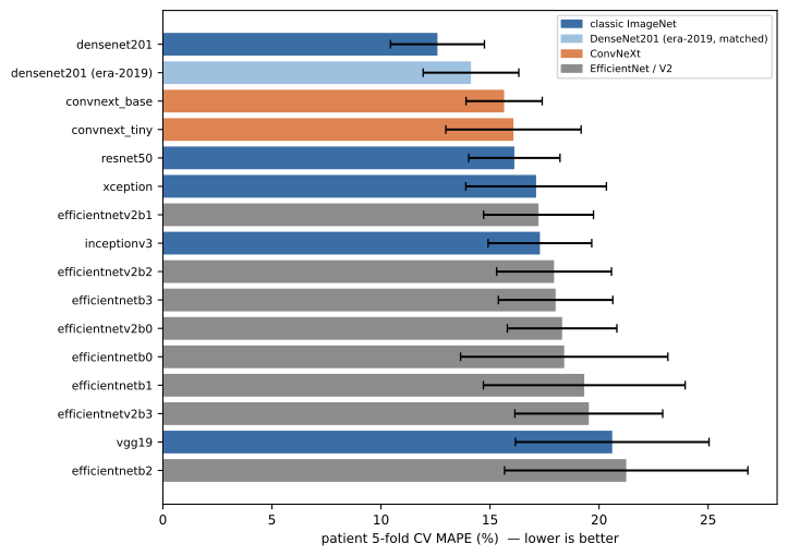
This bake-off, extraction-matched so every row shares one feature-extraction batch, is why DenseNet201 is carried forward: it gives the best \(R^2\), wins the replication, and remains the strongest backbone after tuning. Within the classic group the differences sit inside the per-fold standard deviation, so the ordering should be read against that variance, not as a clean ranking.
Tuning the head on cached features
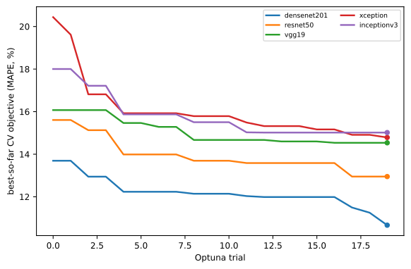
Because the frozen, grid-pooled features can be computed once and cached, the entire hyperparameter search operates on these cached vectors, which makes a large search affordable without a GPU. We tune the head with the Tree-structured Parzen Estimator (TPE) sampler in Optuna, searching over head depth and width, dropout, \(L_2\) weight decay, whether batch normalization is applied, learning rate, batch size, and early-stopping patience. Each protocol is tuned separately — every objective evaluation uses the same sampling protocol it reports, scored on that protocol’s five-fold cross-validation — and a single feature extraction per backbone serves both.
Tuning moves single-model DenseNet201, with frozen and tuned both scored by five-fold cross-validation (mean over folds), from 4.58% to 4.03% MAPE (3.00° MAE) under image-level sampling, and from 12.59% to 10.80% MAPE (8.62° MAE, \(R^2 = 0.886\)) under patient-level sampling. The per-model gains are small but consistent, and they calibrate the five members enough that a plain mean ensemble becomes effective.
The tuned single-model figures are in-sample to the search.
The search selects hyperparameters on the same five folds that are then reported, with no nested or outer test fold, so the tuned single-model numbers are optimistic relative to a held-out set. They are reported as the like-for-like predecessor of the ensemble, not as held-out accuracy.
Figure 3
Five backbones become one estimator
We combine the tuned heads over all five backbones with two combiners: a plain mean of the member predictions, and a stacked generalization in which a Ridge meta-learner is fit on the member outputs. Every reported ensemble figure is computed from out-of-fold (OOF) predictions, pooled across folds into a single metric — under five-fold cross-validation each member predicts only on the fold it did not train on, so under patient-level sampling every ensemble number is evaluated on patients absent from the corresponding fold’s training.
This pooled-OOF aggregation differs from the mean-over-folds aggregation used for the single-model figures, so the two are not strictly the same estimator. Aggregated the same pooled-OOF way, the single tuned DenseNet201 is 7.80° MAE / 10.14% MAPE patient-level — the like-for-like predecessor of the ensemble. Against that anchor, the stacked ensemble’s patient-level gain is genuine and modest: 10.14% → 8.53% MAPE, about a 1.9° improvement in MAE.
The mean ensemble reaches 3.03% MAPE (2.09° MAE, \(R^2 = 0.994\)) image-level and 9.89% (6.89° MAE, \(R^2 = 0.932\)) patient-level. The stacked ensemble — the estimator we carry forward — reaches 2.79% MAPE (1.96° MAE, \(R^2 = 0.995\)) image-level and 8.53% (5.93° MAE, \(R^2 = 0.952\)) patient-level. It is the first configuration to break below 10% MAPE on the cross-patient regime, consistent with the five backbones making partly independent errors.
The Ridge stacker is fit on OOF predictions over only 12 patient groups.
That leaves the meta-layer at some risk of overfitting; no separate nested OOF loop was run for the stacker, so stacking on OOF can be mildly optimistic. We do not report an error-correlation analysis to quantify the members' independence.