Results
Five backbones, two protocols, one ensemble
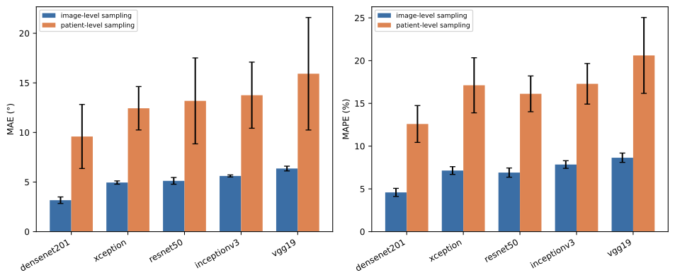
We score the same frozen-feature estimator two ways. Image-level sampling asks how well the model reads the angle across the full population of orientations the augmentation spans; patient-level sampling holds out whole volunteers and asks how well it generalizes to an unseen person. The two answers differ by roughly threefold, and that gap is the result.
The headline is a tuned, stacked ensemble of five frozen ImageNet backbones: 2.79% MAPE / 1.96° MAE / R² 0.995 image-level, and 8.53% MAPE / 5.93° MAE / R² 0.952 patient-level. Below we build to that number from a faithful replication of the EMBC 2019 setup, tune each protocol to its own best, and then take apart what moves the error: the sampling lens, head tuning, ensembling, the choice of backbone, and a classical geometric baseline.
Faithful replication
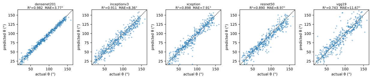
We first reproduce the EMBC 2019 regime: frozen ImageNet backbones with the orientation-preserving grid-pooling head, scored under image-level sampling on the rotation-augmented corpus, with no fine-tuning.
| Backbone (frozen) | MAE (°) | RMSE (°) | MAPE (%) | R² |
|---|---|---|---|---|
| DenseNet201 | 3.77 | 4.75 | 5.84 | 0.982 |
| InceptionV3 | 8.36 | 10.44 | 11.70 | 0.911 |
| Xception | 7.91 | 11.20 | 12.00 | 0.898 |
| ResNet50 | 8.97 | 11.62 | 12.75 | 0.890 |
| VGG19 | 11.67 | 17.77 | 18.01 | 0.743 |
Frozen DenseNet201 reaches 5.84% MAPE / 3.77° MAE, reproducing the regime of the paper’s best single model (≈ 2.87° MAE / 4.03% MAPE) within tolerance and with no fine-tuning. The per-backbone ranking differs from the 2019 study, which reported VGG19 as strongest: with a shared head, pooling, and training budget across backbones, DenseNet201 lands first and VGG19 last here. The replication reproduces the single-digit-degree regime, not the original ordering.
Why this is not yet a real-world accuracy number
This table is image-level sampling on the rotation-augmented corpus, where the 2,100 examples are coupled copies of 84 base images, not 2,100 independent observations. It measures how well the model reads the angle across orientations, not how it generalizes to an unseen patient; for that, read the patient-level column below.The best estimator under each protocol
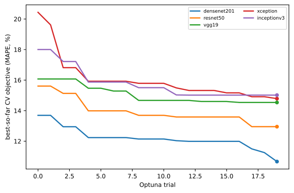
Each protocol is tuned to its own best head and optimizer configuration via Optuna TPE (head depth and width, dropout, L2, BatchNorm, learning rate, batch size, patience), scored on that protocol’s five-fold cross-validation over cached frozen features; a single feature extraction per backbone serves both protocols. Per-backbone rows are five-fold CV means; the ensemble rows are pooled out-of-fold (OOF) over the five tuned models.
| Model (Optuna-tuned) | Image MAE° | Image MAPE% | Image R² | Patient MAE° | Patient MAPE% | Patient R² |
|---|---|---|---|---|---|---|
| DenseNet201 | 3.00 | 4.03 | 0.988 | 8.62 | 10.80 | 0.886 |
| ResNet50 | 3.64 | 4.84 | 0.981 | 9.79 | 13.30 | 0.842 |
| VGG19 | 4.22 | 5.79 | 0.976 | 10.21 | 14.97 | 0.871 |
| InceptionV3 | 4.68 | 6.59 | 0.970 | 10.66 | 14.66 | 0.856 |
| Xception | 4.75 | 6.59 | 0.970 | 10.88 | 14.76 | 0.851 |
| Ensemble (mean) | 2.09 | 3.03 | 0.994 | 6.89 | 9.89 | 0.932 |
| Ensemble (stacked) | 1.96 | 2.79 | 0.995 | 5.93 | 8.53 | 0.952 |
The member rows and the ensemble rows aggregate differently: member rows are per-fold CV means, while ensemble rows are pooled OOF. Aggregated the same pooled-OOF way, the single tuned DenseNet201 is 7.80° MAE / 10.14% MAPE patient-level, the like-for-like predecessor of the ensemble rows; that is the row the ensembling gain should be read against.
The scatter below pairs the stacked ensemble’s predictions against the reference angle, image by image.
Two protocols, two questions
Holding the frozen grid-pooling model fixed and changing only the sampling protocol, every backbone loses accuracy under the stricter cross-subject split, by margins that separate the backbones cleanly.
| Backbone (frozen) | Image MAPE % | Image R² | Patient MAPE % | Patient R² |
|---|---|---|---|---|
| DenseNet201 | 4.58 | 0.987 | 12.59 | 0.869 |
| ResNet50 | 6.90 | 0.964 | 16.12 | 0.738 |
| Xception | 7.14 | 0.967 | 17.11 | 0.784 |
| InceptionV3 | 7.85 | 0.959 | 17.29 | 0.743 |
| VGG19 | 8.64 | 0.942 | 20.60 | 0.626 |
The tuned stacked ensemble reaches 2.79% MAPE / 1.96° MAE under image-level sampling and 8.53% / 5.93° under patient-level, roughly a 3× MAPE spread. This is the expected signature of a small cohort (~10 volunteers): the model interpolates the augmented-image manifold very well, while cross-subject generalization is intrinsically harder and carries genuine per-fold variance. DenseNet201 holds both the smallest protocol gap and the highest patient-level R² (0.869), which is why it is carried forward; the ordering among the weaker four shifts with the lens, while the choice of lead backbone does not.
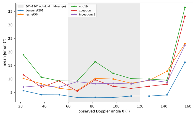
The same protocol gap shows up as a function of the true angle: error grows toward the extreme insonation angles, where the geometry is least forgiving.
Frozen versus tuned
Tuning the head helps under both protocols. For DenseNet201, like-for-like under five-fold CV against the grid-pooling frozen baseline: image-level 4.58% → 4.03% MAPE and patient-level 12.59% → 10.80%. The gains are modest per model but consistent, and tuning makes the five members well-calibrated enough that a plain mean ensemble works, where an untuned mean ensemble was effectively useless.
Ensembling is the biggest lever
Ensembling moves the error more than any single other choice. Best single model to stacked ensemble: image-level 4.03% → 2.79% MAPE (3.00° → 1.96° MAE) and patient-level 10.80% → 8.53% MAPE (8.62° → 5.93° MAE). Read against the like-for-like pooled-OOF predecessor, the single tuned DenseNet201 at 7.80° MAE / 10.14% MAPE patient-level, the genuine ensembling gain is about 1.9°.
The five backbones make partly independent errors, so combining them — a plain mean, or a Ridge stacker over OOF predictions — recovers accuracy a single model cannot. Under the honest patient-level protocol, the tuned stacked ensemble is the first configuration to break below 10% MAPE (8.53% pooled OOF), improving on the untuned ensemble.
Stacking on out-of-fold predictions can be mildly optimistic
The ensemble rows are pooled out-of-fold predictions, and the Ridge stacker is fit on those same OOF predictions. This reuse can make the stacked number mildly optimistic relative to a fully nested protocol, so the 8.53% patient-level figure is best read as an upper-bound-leaning estimate rather than a guaranteed held-out accuracy.
Newer is not better
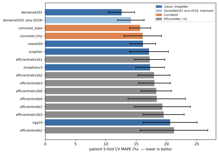
A frozen bake-off under patient five-fold CV (grid pooling, untuned heads) spans the classic ImageNet encoders and the modern ConvNeXt and EfficientNet families. The classic backbones clearly beat the modern ones.
| Tier | Backbones | MAPE (%), patient 5-fold |
|---|---|---|
| Classic ImageNet | DenseNet201 (best, 14.13), ResNet50, VGG19, InceptionV3, Xception | ~14 |
| ConvNeXt | ConvNeXt-Base (15.65), ConvNeXt-Tiny (16.07) | ~16 |
| EfficientNet / V2 | B0–B3 and V2-B0–B3 families | ~17–21 |
Within the classic group the differences sit inside the per-fold standard deviation; across families, the older encoders win. Every row in this bake-off shares one feature-extraction batch, so DenseNet201’s 14.13% here is the like-for-like point against the modern backbones, whereas its replication-extraction value above is 12.59%. With only 84 base images, larger and ImageNet-stronger encoders have nothing to grip. DenseNet201 — the best R², the replication winner, and the strongest after tuning — is carried forward.
One backbone was extracted on a different runtime
ConvNeXt fails to run on TF-Metal because of an XLA op-support gap, so it was extracted on JAX-CPU. The bake-off otherwise shares a single feature-extraction batch per row, which is why DenseNet201's bake-off value (14.13%) and its replication-extraction value (12.59%) differ.Learned versus classical, and fusion
A purely classical, image-only structure-tensor angle prior reaches 3.16° MAE on the narrow base-angle band, and a circular fusion of the learned and classical estimates reaches 2.72° MAE, improving on the classical prior and on the learned model’s base-band error. The learned model and a hand-crafted geometric cue capture partly complementary information.
The fusion number is in-sample, on a narrow band of angles
The 3.16° structure-tensor and 2.72° fusion figures are computed in-sample on the narrow band of base angles, not on a held-out split, and they are recomputed at runtime rather than stored inresults/. They show that classical geometry carries complementary signal, not that fusion is a validated held-out improvement.