Classifying galaxy morphology with a CNN

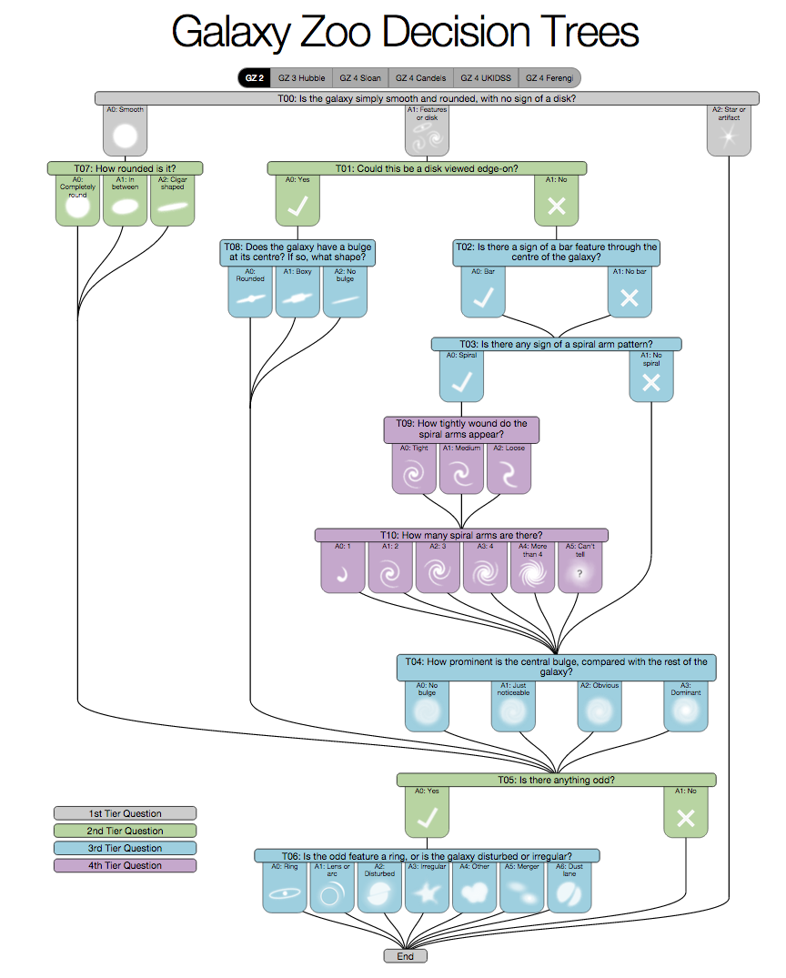
Since 2007, thousands of volunteers have looked at 100k+ galaxy images and answered a tree of questions about each one: is it smooth or does it have features, is there a spiral, how many arms. The answers for each galaxy get collapsed into 37 numbers, a record of what a crowd of human eyes saw. That record is what makes this a tractable supervised-learning problem in the first place. The build question I want to settle here is narrow and concrete: can a convolutional net reproduce those same 37 numbers from raw pixels, with no astronomer hand-crafting a single feature along the way? I am going to assemble the network one piece at a time and explain what each piece is for as it goes in. There is no trained accuracy or loss in this post. The content is the architecture and the data, not a benchmark, and the loss curve is the next post.

So rather than walk a single image straight through and narrate whatever it hits, I want to put the finished machine on the table first and then take it apart. Here is the whole pipeline, the thing every later section will be adding a labeled part to.

That is the whole of it. Every section below picks one labeled box out of this diagram and explains what it does and why it has to be there, starting from the block on the far left and ending at the strip of 37 numbers on the far right. The single image I follow through the network is the running thread that ties those boxes together, so before I touch any layer I should be precise about what that image actually is and where it comes from.

The data comes from the Sloan Digital Sky Survey, the imaging project behind the citizen-science effort. To quote the SDSS site:

The Sloan Digital Sky Survey has created the most detailed three-dimensional maps of the Universe ever made, with deep multi-color images of one third of the sky, and spectra for more than three million astronomical objects.

The volunteer scoring happened through Galaxy Zoo, launched in 2007, where thousands of people classified 100k+ images of galaxies by walking a decision tree of questions.

The input box: a 424x424x3 jpeg and a 37-vote vector

The leftmost block in the pipeline is the input, and the rightmost strip is the target. Pin down both ends first, before anything in between exists. The dataset is 100k+ jpeg images plus, for each image, a score vector with 37 values, where each value is the weighted score from volunteers on one question in the tree.

These targets are not probabilities, which is the first thing that shapes the design of the box at the far right. They are weighted vote scores, so each value runs from 0 to 1, but the sub scores for a single question do not necessarily sum up to 1. That detail decides the loss and the output head later, and I will come back to it once the diagram has grown that far.

Every image is 424×424×3 and each value sits between 0 and 255. Before the image hits the network I rescale it, computing $\mu_\text{channel}$ and $\sigma_\text{channel}$ over the full dataset and then normalizing each channel using its own $\mu$ and $\sigma$. The channels and cell values here do not carry physical meaning. They are standardized to the 0-255 image range, so this normalization is a gradient-update convenience, not a domain-informed transform.

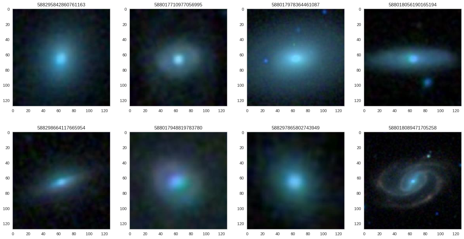
Once I pick one of those galaxies, it is read into Python as a numpy array, and that array is the literal substrate every box downstream operates on. Here is what the input block in the pipeline diagram unfolds into.

The output box: why regression, not classification

The rightmost box in the pipeline is a regression head rather than the classifier you might expect, and it is the box whose shape the input data dictated. Pin it down before I fill in the conv stack between the two ends. A convolutional network reads the image array, builds up features from it, and emits an output. The usual classification setup uses a one-vs-rest encoding, where the correct class is assigned 1, every other class is assigned 0, and the output is a vector of length c for c classes. That is clean, but it assumes there is one right answer per image.

That assumption does not hold here, because the ground truth is a weighted vote vector rather than a single label, so I set this up as a 37-dimensional regression instead. The network outputs a vector of length 37 and is trained to match the human vote scores directly, sub-1 sums and all, which means the target shape dictates the head: 37 continuous outputs, linear, no softmax. My first pass reflexively reached for a softmax over the 37 outputs. That is exactly wrong here: softmax does not leave the votes alone, it renormalizes the whole vector to sum to 1, and the votes do not.

With both ends of the pipeline now nailed down, a 424x424x3 array on the left and 37 linear outputs on the right, the rest of the diagram is the stack of layers that carries one into the other.

The conv and pool blocks: what each one does to our image

The normalized array flows through the chain of conv-and-pool blocks in the middle of the diagram, shrinking as it goes, and each block is really two distinct operations worth separating. Here is what each one does to the array as it passes through.

The convolutional layer is where the learned features live. In a classic modeling pipeline the features are hand-crafted, with an expert deciding which transforms of the raw input matter, and the convolution kernels replace that step entirely. They are fit against the target, so instead of an astronomer choosing what counts as a spiral arm, the kernels learn whichever filters best drive the 37-value prediction.

The pooling layer shrinks the representation, which is the part of the block that accounts for the diagram’s boxes getting smaller from left to right. max-pooling keeps the largest value in each window as the summary of that region and average-pooling keeps the mean, but either way the spatial footprint goes down while the salient signal survives, which leaves fewer spatial positions for the next conv block to scan over.

The activation introduces nonlinearity by applying a function elementwise to the array, and which function it is depends on where it sits in the diagram. I use relu between conv blocks to keep gradients flowing, while the output head stays linear because this is regression onto continuous vote scores rather than a softmax over mutually exclusive classes. Softmax would force the 37 outputs to sum to 1, and these vote scores do not.

That is the visible skeleton of the pipeline. Two more pieces ride inside these blocks without showing up as their own boxes in the diagram, dropout and batch normalization, and each of them earns its own section.

Batch normalization between the blocks

The first of the two hidden pieces sits between the conv blocks, and the reason it needs to be there is something that only shows up once training is underway. As training proceeds, the parameters of earlier layers keep changing, so the distribution of inputs landing on each later layer keeps moving underneath it. Ioffe and Szegedy called that moving target internal covariate shift, and argued it pushes you toward small learning rates to keep things stable. Whether that is the precise reason batch norm helps has since been debated, but the fix is the same: batch normalization normalizes each channel’s activations to $\mu_x = 0$ and $\sigma_x = 1$ across the current mini-batch, then applies a learned affine transform.

Here $\mu_X$ and $\sigma_X$ are computed channelwise, the same axis I standardized the raw pixels along at the input, except now it happens between conv blocks in this stack and the statistics come from the live mini-batch instead of the whole dataset. With the input distribution re-centered, downstream layers see something stable to learn against, which is what buys back the larger learning rates and faster training than the same network without batch normalization.

Dropout on the dense head

The second hidden piece lives at the far end of the diagram, on the dashed dense box just before the 37-value strip, which is where the parameter count is highest and overfitting bites first. Dropout is a regularizer for overfitting, and in this build it sits exactly there. At training time, the activations of a randomly chosen fraction of units are set to zero, and at test time every unit is kept, with its activations scaled by the keep-probability p so the expected magnitude matches what later layers saw during training. Because a different random subset is dropped at each step, no single unit can carry the representation on its own, so the dense head is pushed to spread the 37-value prediction across many units.

The assembled network and what I would watch next

With every box in the diagram now labeled, the input array on the left, the conv-and-pool blocks shrinking through the middle, batch norm sitting between them, dropout on the dense head, and the 37-value regression head on the right, the layers stack into a module that I can sweep across several network structures. I start from a VGG-style stack of small 3x3 convolutions and move toward residual ResNet-style blocks. The hope with the deeper residual variants is that skip connections let me add depth without the gradient dying on the way back, which matters when the head has to resolve 37 separate vote scores rather than pick one class. The final layers are Dense (fully connected), and their output is compared against the expected 37-value vector to compute a per-observation loss, which is back-propagated to update both the convolutional kernels and the dense weights.

Looking back over the assembled diagram, the wider point is that the convolution kernels in the middle stand in for an astronomer’s hand-crafted features: nobody encodes what a spiral arm looks like, and the filters are fit against the votes instead. The limit is just as plain, because everything I have drawn here is the data and the architecture, the setup for the experiment, and it deliberately stops short of a trained accuracy or a final loss. The number I want to watch first, once the diagram is trained, is the gap between train and validation MSE on the 37-value vector, which is where the dropout on the dense head earns its place or does not. What this whole diagram leaves on the table is the framing itself, 37 numbers that humans voted on, predicted straight from a 424x424x3 jpeg.

References

1. Srivastava, N., Hinton, G., Krizhevsky, A., Sutskever, I., and Salakhutdinov, R. (2014). Dropout: A Simple Way to Prevent Neural Networks from Overfitting. Journal of Machine Learning Research, 15.
2. Ioffe, S. and Szegedy, C. (2015). Batch Normalization: Accelerating Deep Network Training by Reducing Internal Covariate Shift. Proceedings of the 32nd International Conference on Machine Learning.