
Training a model once is cheap. The expense is in tuning it: you do not fit one model, you fit a few hundred, one for every combination of settings, and keep whichever scored best. Those fits do not depend on each other. The search is embarrassingly parallel, the same shape as the feature loop in the first post, and it runs on the same Dask cluster the same way.
The interesting part is that you do not have to run all of it. dask-ml, the machine-learning toolkit built on Dask, has a search for exactly this, called Hyperband: it spends most of its budget on the configurations that are doing well and pulls the plug early on the ones that are not. That is what this post is about, not making any single fit faster, but skipping the fits that were never going to win.
This is the second half of a small Dask project, and it opens with the model that nearly convinced me Dask had no place here.
In the first post I turned about 5,200 LINEAR light curves into a feature table, one row per star, twelve numbers each. The astroML catalogue also ships four colours per star (ug, gi, iK, JK), so I bolted those on too, for sixteen features total. Hand that table to a random forest and it sorts the five star types at 96.8% on a held-out quarter, with no tuning whatsoever. The colours earn their place: drop them and accuracy falls by about a point, from 96.8% to 95.7%.
So the classifier is done. A random forest with default settings is hard to beat on a table this size, and it has no knobs I need to touch. Which leaves the actual question this post is about, the one the forest is too easy to show: when a model does need its knobs set, how do you set them without wasting most of your compute? Because the standard answer wastes a lot.
This is not about making the forest faster (it fits in two seconds, leave it alone) or about data that does not fit in memory (it fits). It is about the search, run on a model that genuinely needs searching, with a Dask-native method that gives up on the bad configurations early.
A model that actually needs tuning
The forest is the wrong thing to study tuning on, for two reasons: it barely needs it, and it trains in one shot, so there is nothing to watch. I want the opposite. A plain linear classifier trained by stochastic gradient descent gives me both.
from sklearn.linear_model import SGDClassifier

clf = SGDClassifier(loss="log", penalty="elasticnet", tol=1e-3)
# learns one pass at a time:
for _ in range(n_epochs):
    clf.partial_fit(X_train, y_train, classes=classes)
This is multinomial logistic regression, fit by SGD. On the scaled sixteen features it reaches about 92%, a few points under the forest, but it has the two properties the forest lacks. It is genuinely sensitive to its regularisation: the alpha and l1_ratio knobs move its accuracy around by several points, so the tuning is not cosmetic. And it learns incrementally, one partial_fit pass at a time, so I can train it a little, look at how it is doing, and decide whether to keep going. That second property is the whole game here.
The default: train everyone to the end
The standard way to set alpha and l1_ratio is to sample a few hundred combinations, train each one to convergence, and keep whichever scored best. Random search. It is trivially parallel, one independent fit per configuration, exactly the shape from the first post, so I ran it the same way, 143 configurations as dask.delayed tasks across eight workers.
Here is what that costs. Each of the 143 configurations trains for 81 epochs. That is 143 x 81 = 11,583 training passes. On the cluster the whole search finished in 8.3 seconds, at a best test accuracy of 92.5%.
The number that bothers me is 11,583. A configuration with a hopeless learning rate, or so much regularisation that it underfits, is recognisable as a loser after five or ten epochs: its validation score is bad and not moving. Random search trains it for all 81 anyway, then throws the result away. Most of those 11,583 passes were spent finishing models that were already out of contention.
Give everyone a little, then cut
The fix is an old idea with a good name: successive halving. Give every configuration a small budget, say one epoch. Look at the scores. Keep the top third, throw the rest away, and give the survivors three times the budget. Look again, cut again. After a few rounds, only a handful of configurations are still standing, and those are the ones getting trained to the full 81. The bad configurations died cheap.
Successive halving has one awkward knob of its own: how aggressively to cut, and how many configurations to start with. Cut too hard and a slow starter that would have come good never gets the epochs to prove it; cut too gently and you have just rebuilt random search with extra steps. Hyperband is the trick that removes that knob: it runs several successive-halving brackets side by side, each with a different starting count and cut rate, so it hedges across the aggressive and the cautious schedules instead of betting on one. You get the early-stopping savings without having to guess the schedule.
Hyperband on the cluster
dask-ml ships Hyperband as a drop-in search, and on a cluster it has a nice property: the brackets, and the models within them, are independent, so the scheduler runs them across the workers the same way it ran the feature loop in the first post. The only constraint is the one from earlier, the estimator has to support partial_fit, which is why this is the SGD classifier and not the forest.
from dask_ml.model_selection import HyperbandSearchCV
from scipy.stats import loguniform, uniform

params = {"alpha": loguniform(1e-6, 1e-1), "l1_ratio": uniform(0, 1)}
search = HyperbandSearchCV(clf, params, max_iter=81, aggressiveness=3)

with Client(cluster):
    search.fit(X_train, y_train, classes=classes)
max_iter is the most epochs any single model can earn, and aggressiveness sets the cut rate. The search figures out the bracket schedule from those two numbers. Watching the dashboard while it runs is the clearest picture of what it does: models appear, most of them run for a few epochs and vanish, and a thinning set keeps going.
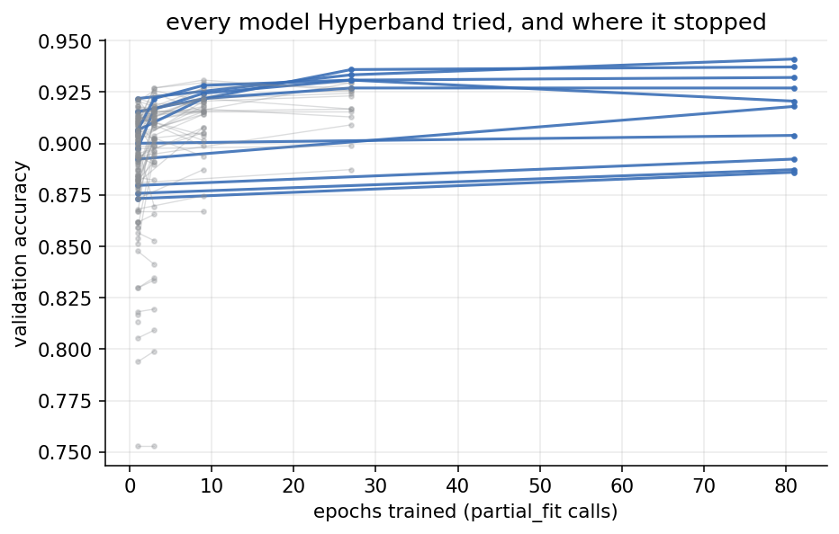
What the early stopping bought
Same 143 configurations explored, two ways to spend the epochs:
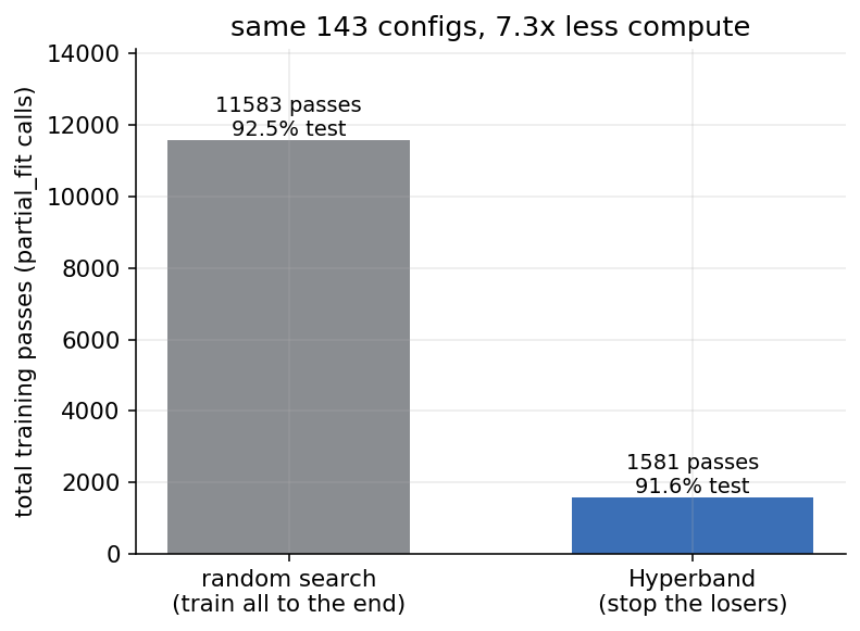
Random search spent 11,583 training passes to find its best configuration. Hyperband explored the same 143 configurations in 1,581 passes, 7.3x less compute, because it stopped the losers after a rung or two instead of training them to the end. On the test set it landed at 91.6% against random search’s 92.5%. That gap is about a dozen of the 1,301 test stars, and it is one run on one seed, so I read it as a tie rather than a loss. On the validation score the search was actually optimising, Hyperband’s pick was the better of the two.
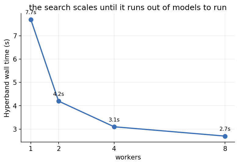
On eight workers that compute saving is a wall-clock saving too: the Hyperband search finished in about 2.7 seconds against random search’s 8.3. The search itself parallelises across configurations, so adding workers helps until there are no more models to run at once:
Where this stops being the answer
Hyperband only helps a model you can stop and restart, one that learns a bit at a time. The random forest has no partial_fit: there is no half-trained forest to judge after one epoch, so none of this applies to it, and you are back to plain random search if you want to tune one. And the forest is still the better classifier here, 96.8% against the tuned linear model’s 91.6%. For a table of sixteen features, the forest wins and barely needs tuning; the search lesson only shows up because I picked the model that does.
The other limit is scale. On this problem the absolute saving is seconds, because an SGD epoch on four thousand rows is nearly free. The reason to care is what happens when an epoch is not free: tuning a gradient-boosted model with hundreds of rounds, or a neural net with real epochs, where a single bad configuration trained to the end costs minutes. There the 7.3x is minutes saved per search, and the same HyperbandSearchCV call scales out across a cluster without changing a line. That is the case I would actually reach for it, and the one I will try next.
dask-experiments on GitHub Part one: the feature loop When the model itself outgrows one machine