
Dask is a library for running generic Python & its data ecosystem libraries in parallel. The core advantage is that you do not rewrite your code as a parallel program. You keep NumPy, pandas, the plain functions you already have, and Dask works out how to spread the work across your cores, or across a whole cluster, and runs it for you.
It comes in a few pieces, and the first job was sorting out which one I actually needed. dask.array and dask.dataframe stand in for NumPy arrays and pandas frames when the data is too big to hold in memory. That was not my first problem; my data fit fine on a single instance. My problem was a slow loop over things that fit, and the piece for that is dask.delayed: it takes the function calls you would have written in the loop and records them as a graph of tasks the scheduler can run in parallel. No out-of-core machinery, no rewriting the science. That small corner of Dask is the whole of this post, and the arrays and bigger-than-memory tricks can wait for another day.
To learn it properly instead of skimming the docs and forgetting them, I took a real problem using data from the LINEAR survey.
I took about 5,200 light curves, one CSV per star, real ones from the LINEAR survey, and set up a script that turned each into a row of features. It was also doing the most frustrating thing a program can do - pinning one CPU core at 100% while the other seven sat at zero, for almost five minutes, on work where every star is independent of every other one. Each star is independent of the other, so e.g. nothing about star number 5,000 depends on star number 4,999. No ordering, no shared state, no reason to do them one at a time except that a for loop is the first thing your fingers reach for. Embarrassingly parallel work, and I was grinding through it one core at a time.
The fix comes to two lines, and one decision in them is which Dask scheduler you hand the work to.
What the loop was doing
The light curves are real, from the LINEAR survey, packaged by astroML with hand-checked class labels. Five kinds of star are in here: RR Lyrae of both the ab and c types, the two flavours of eclipsing binary (close contact pairs and the deeper Algol type), and a thin scattering of Delta Scuti. Each star is a string of brightness measurements on the irregular cadence a real survey actually produces, a hundred to a few hundred points spread across years, with the gaps you get from weather and daylight.
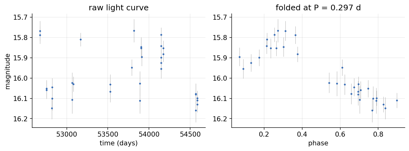
The per-star job is to read the file and boil the light curve down to a fixed vector of features: a period, an amplitude, a few shape and scatter statistics. The slow part is the period. To find it you run a Lomb-Scargle periodogram, which scans close to a hundred thousand trial frequencies across the multi-year baseline and asks how well each one explains the data. That scan is most of the per-star cost, and it is pure CPU.
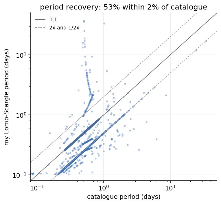
Does the expensive step even produce the right answer? The LINEAR catalogue ships its own validated periods, so I can hold mine up against them:
Here is the unit of work, in full. It is not interesting, and that is the point:
def features_for_file(path):
    """Read one light-curve file and return its features as a dict."""
    t, m, e = read_light_curve(path)
    row = {"star_id": star_id_from_path(path)}
    row.update(extract_features(t, m, e))
    return row
And here is the loop I started with, the baseline:
rows = [features_for_file(p) for p in paths]
On my machine that list comprehension is about 56 ms per star, and across all 5,204 it takes 294 seconds, just under five minutes. One core the whole time.
dask.delayed: stop calling the function
dask.delayed is a decorator that turns a normal function call into a promise to call it. When you wrap features_for_file in delayed and call it, nothing runs. Instead Dask records a little node: “here is a function, here is the argument, here is where the result will go.” Do that for every file and you have not computed anything yet. You have built a graph.
import dask

tasks = [dask.delayed(features_for_file)(p) for p in paths]
tasks is now 5,204 unstarted nodes. The function inside them is byte-for-byte the same features_for_file from above. I did not rewrite the science to parallelize it. I wrapped the call and stopped running the loop myself.
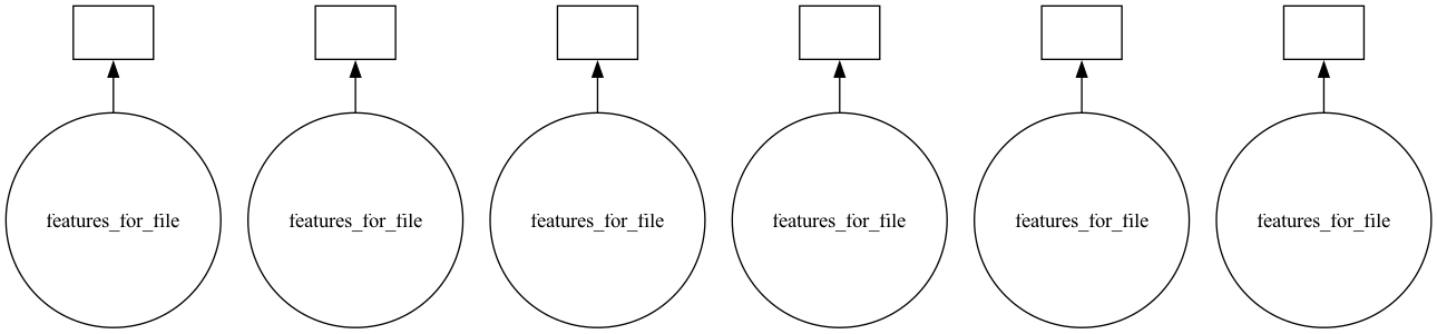
The shape of this particular graph is the simplest one there is: a row of independent leaves with nothing connecting them, because no star needs any other star’s result.
You can see this for real on a handful of files. dask.visualize renders the graph Dask built:
dask.visualize(*tasks[:6])
A cluster on one machine and a dashboard to monitor it
A graph is just a plan. To run it you hand it to a scheduler. The one I want is the distributed scheduler, because it comes with two things I care about: real worker processes, and a live dashboard.
from dask.distributed import Client, LocalCluster

cluster = LocalCluster(n_workers=8, threads_per_worker=1)
client = Client(cluster)
LocalCluster starts eight worker processes on this one machine. Client connects to them and, as a side effect, prints a dashboard URL. Open it and you get the single most useful thing about Dask: a real-time picture of what the workers are doing.
results = dask.compute(*tasks)
compute is where those promises actually run. It ships the graph to the scheduler, which starts handing tasks to whichever workers are free, and the dashboard fills in.
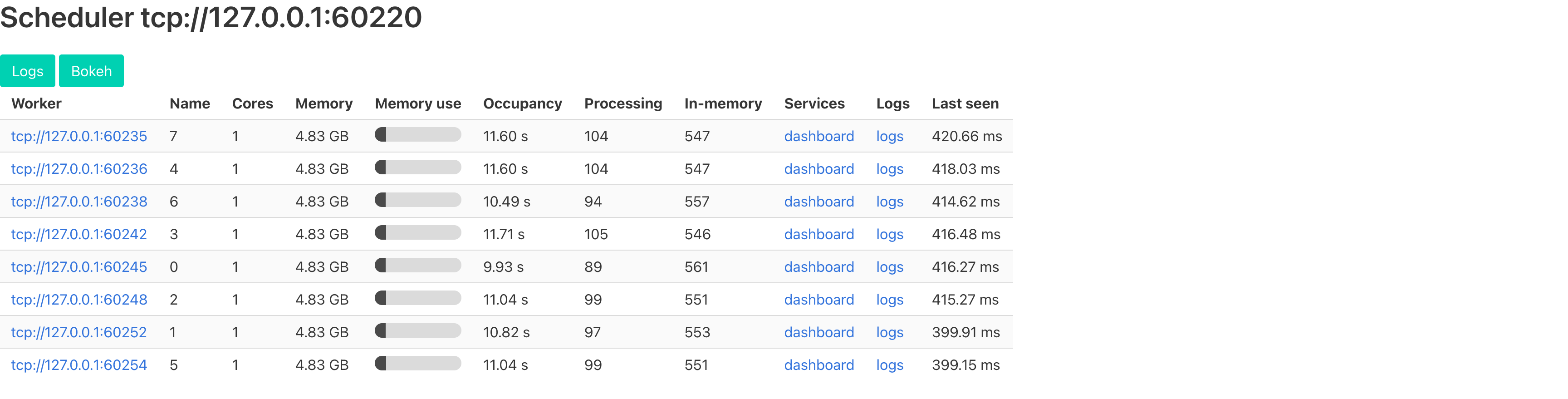
The first time I opened the dashboard mid-run, Dask stopped being something I had to take on faith. Eight Processing counters sitting near a hundred is the whole story: the workers are busy, in parallel, and I can watch it happen instead of inferring it from a stopwatch at the end. When a run goes wrong the same view shows it in a couple of seconds, one worker buried and the other seven idle.
Eight workers, three and a half times faster
Here is the full run, the same 5,204 stars, three ways:
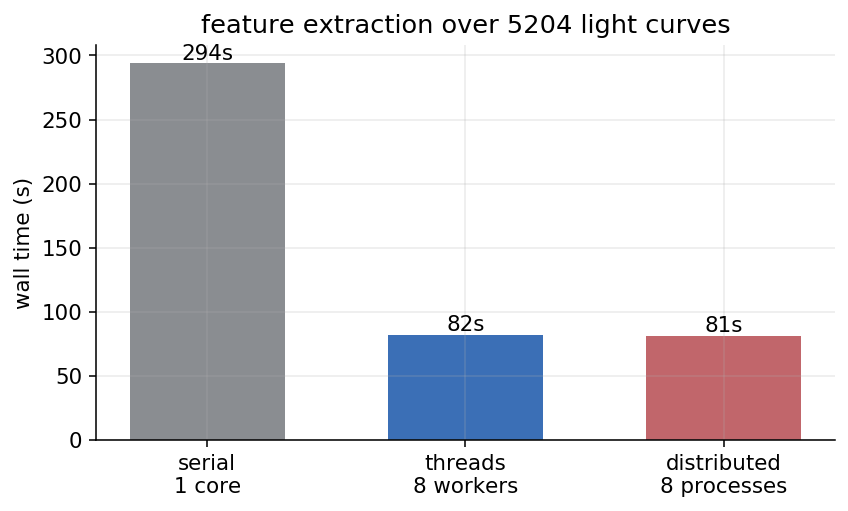
The serial baseline was 294 seconds. The distributed scheduler on eight worker processes did it in 81, which is 3.6x. The first thing to say about that number is that 3.6 is not 8. Eight workers did not come close to making it eight times faster, and where the rest went is the more interesting part of this section.
But the number I did not expect was the middle one. Dask has a threaded scheduler too, and switching to it is a one-line change:
dask.compute(*tasks, scheduler="threads", num_workers=8)
Eight threads instead of eight processes. I went in assuming Python’s global interpreter lock would wreck it, because the GIL lets only one thread execute Python at a time and “use threads for CPU work in Python” is usually a trap. It came in at 82 seconds, 3.6x, a single second behind the worker processes. One second out of 82 is well inside the run-to-run noise, so I read threads and processes as a flat tie, on a workload I had written off as hopeless for threads.
The reason is that almost none of the per-star cost is Python the GIL can block. The Lomb-Scargle periodogram, and the astropy and NumPy underneath it, are compiled code that releases the GIL while it runs, so eight threads genuinely compute eight periodograms at the same time. The only thing left holding the GIL is the pandas read for each file and the small dict I build at the end, and on these light curves, where each periodogram chews through a few hundred points, that residue is too small to measure. So worker processes, which do not share a GIL at all, have essentially nothing to win back. Threads and processes tie.
So neither half of my mental model survived the stopwatch. For this workload the two schedulers tie, and the way you learn that is the dashboard and a stopwatch, not a rule of thumb.
That still leaves the bigger gap. Eight workers, 3.6x. I did not profile where the missing speedup went, but the shape is familiar: 5,204 files means 5,204 tiny reads, which is I/O rather than CPU and does not split cleanly across cores, and each task runs for only about 56 ms, short enough that the scheduler’s own bookkeeping starts to show against it. This is not the long, pure, CPU-bound work that scales to a clean 8x.
That last part has a knob I left alone here but would reach for next. When tasks are too small, you batch them: hand each task a list of files instead of one, and let it loop internally, so the per-task overhead is amortised over fifty stars rather than paid for each.
def features_for_batch(paths):
    return [features_for_file(p) for p in paths]

chunks = [paths[i:i + 50] for i in range(0, len(paths), 50)]
tasks = [dask.delayed(features_for_batch)(c) for c in chunks]
The arithmetic does not change and neither does the worker count, but now the scheduler tracks a hundred fat tasks instead of five thousand thin ones. On work this short that is the difference between fighting the overhead and ignoring it.
What this bought, and what it did not
The accounting: I turned a five-minute serial loop into an 81-second one by changing two things. I wrapped one function in dask.delayed, and I picked the distributed scheduler. The science code did not change at all.
What Dask did not do is make anything faster on a single core, or rescue an algorithm that was badly written. The per-star work is identical; there is just more of it happening at once. If features_for_file had been slow because of a bad inner loop, Dask would have faithfully run that bad loop on eight workers and I would have learned nothing. Parallelism is a multiplier on the work you have, not a fix for the work being wrong.
And it is not free. The distributed scheduler spends real time spinning up workers, pickling your functions, and shipping results back. On 5,204 stars that overhead disappears into the win. On a handful it would dominate, and the plain for loop would beat all of this. The break-even is real: reach for a cluster when the pile of independent work is genuinely large.
That is the embarrassingly-parallel case in one move: the unit of work does not depend on its neighbors, so you wrap it and hand the scheduler the pile. The code that does this lives in the companion repo, the same one these light curves come from.
dask-experiments on GitHub Dask project site
The next thing I wanted was to actually use these features: feed them to a classifier and see whether a machine can tell an RR Lyrae from an eclipsing binary the way the periodogram quietly already did. That turned into a second post, where the data fits in memory easily and the model trains in seconds, so the thing Dask speeds up is the hyperparameter search around it, most of which turns out to be wasted on configurations that lost in the first few epochs.