The UCI Human Activity Recognition data gives you 561 numbers for every 2.56 seconds a phone spends strapped to someone’s waist. Thirty volunteers between 19 and 48 wore one while they walked, climbed stairs, sat, stood and lay down, and the project’s authors turned each window of raw acceleration into 561 time domain and frequency domain features. That is a generous description of six activities, and my working assumption was that a phone asked to compute all of them continuously would spend its battery doing it. The question I took into this project was how few of the 561 a classifier actually needs.
The answer is five. It took two passes to find them, because the first importance ranking I computed points at a different five.
The file I modeled is the training partition
The file I worked from is a slice of that 30 volunteer experiment. It is samsungData, an .rda, and the notebook markdown records what it holds: the combined form of all files in the train folder. That is the UCI training partition, 7352 windows from 21 of the 30 subjects. The remaining nine volunteers live in the test folder and never enter anything below.
R objects and pandas do not get along, so I converted the .rda into a pipe separated text file and loaded that.
data = pd.read_csv('../data/samsungData.txt',sep='|')
data.head()               # 5 rows x 563 columns
data.activity.unique()    # standing, sitting, laying, walk, walkdown, walkup
563 columns: the 561 features, a subject id, and the activity label. The classes are uneven without being lopsided: laying 1407 windows, standing 1374, sitting 1286, walk 1226, walkup 1073, walkdown 986, the smallest at 70 percent of the largest. pandas_profiling wrote a data_profile.html over the frame and reports no missing values; I took its word for that rather than checking the columns myself. The features also arrive normalized, every pairplot axis near the end of this post runs the same -1 to 1 range, so nothing below involves imputation or scaling.
All of it runs on the university cluster’s Intel Python 2.7 build, with n_jobs=4 in every forest. The notebook imports matplotlib.pyplot twice, which tells you roughly how carefully it was assembled.
561 features do not span 561 dimensions
Every one of the 561 columns is derived from the same handful of raw acceleration streams, so a lot of them have to be measuring the same thing in slightly different words. The correlation matrix confirms it.
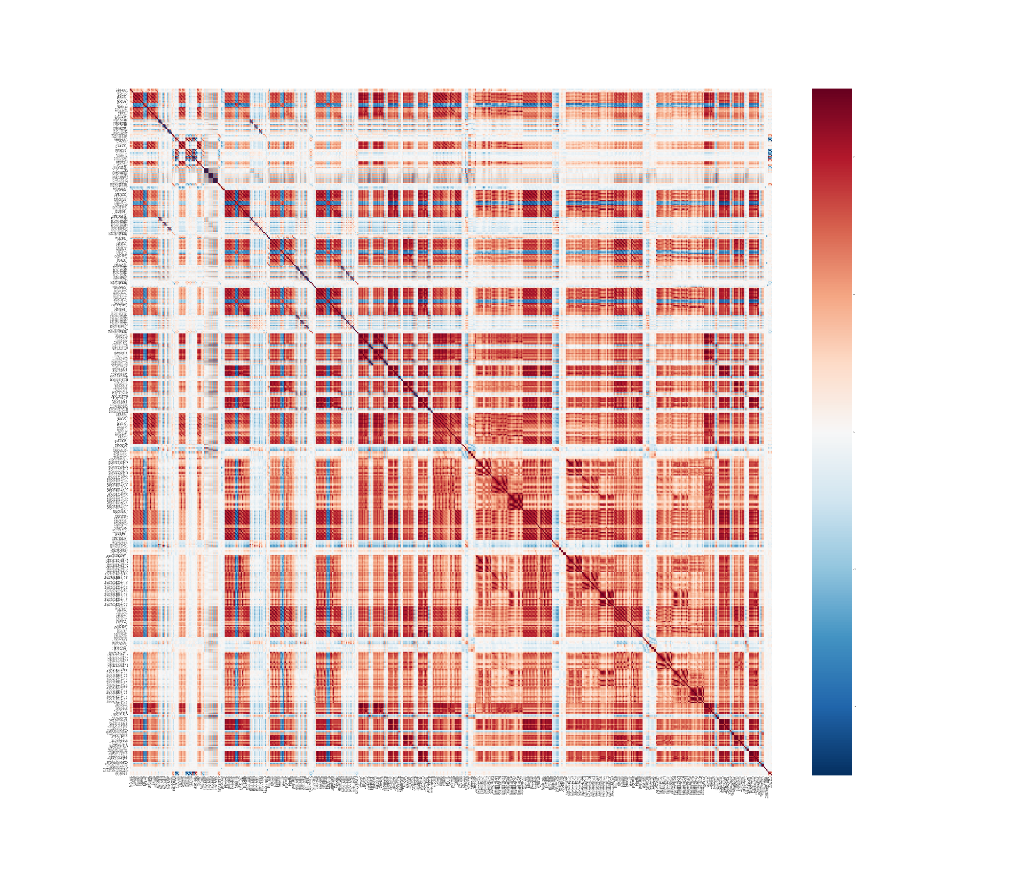
The variance table says the same thing from the other end. Sorted ascending, its bottom rows are features that barely move at all: tGravityAcc-iqr()-X at 0.005378, tBodyAcc-mean()-Y at 0.001665. A column that does not vary cannot separate anything.
Plotting per-activity distributions for 561 features is not an activity I recommend, so I looked at a handful. tBodyAccJerk-std()-X is representative.

tBodyAccJerk-std()-X by activity, one panel each. Laying, sitting and standing pile up at the low end; walk, walkup and walkdown spread higher.A principal component still needs all 561 features
The textbook move against correlated columns is PCA, so I ran it: sklearn PCA with n_components=561, fit on all 561 feature columns. The first component alone explains 0.625544 of the total variance and the top five together explain 0.751587, which is about what the correlation blocks led me to expect.
002.PCA.ipynb ends on a bar chart of the top twenty components with a cumulative line and no conclusion written under it. A principal component is a weighted sum of all 561 features, so a five component model still needs the phone to compute all 561 numbers before it can project them down. tBodyAccJerk-std()-X is a column I can compute on a phone and describe in a sentence; the first principal component of this partition is something I can compute on a phone and describe to nobody.
Splitting by record leaks near twins across the boundary
Everything below runs off one 70:30, train/test split
randomState = 42

train = data.sample(frac=0.7, random_state=randomState)
test  = data[~data.index.isin(train.index)]

len(train), len(test)     # 5146, 2206
That draw is by record, not by subject, and I want the cost of that on the table before any accuracy lands. Each record is a 2.56 second window and consecutive windows overlap by 50 percent, so two neighbouring records share half their raw samples. Sample at random and one of a pair goes to train while its near twin goes to test, and all 21 subjects have windows on both sides of the line. UCI ships a subject-wise split for exactly this reason. Mine ignores it.
For tuning I used the out of bag score - each tree in a random forest trains on a bootstrap sample of the rows, and the rows left out are a held out set for that tree. Average across the forest and you get a validation number during training, for free, without touching the 2206.
The top five of the first ranking reach only 85 percent
The first model takes all features as-is :
ntree = 25

model0 = rfc(n_estimators=ntree, random_state=randomState, n_jobs=4,
             warm_start=True, oob_score=True)
model0.fit(train.ix[:,:-2], train.activity)

model0.oob_score_         # 0.96502137582588421
That is the reference to beat, and more usefully it is a ranking : a fitted forest reports how much each feature contributed to its splits, averaged over every tree.
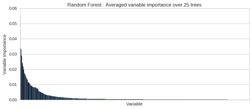
No single feature is worth much on its own here.
With the ranking in hand, the obvious next step is to keep the top k and see how far down the list I can cut. model1 is the same forest with warm_start off and the same seed, retrained from scratch on the top k features by model0’s importance, for k from 1 to 25. I also swept the tree count, so that knob first.
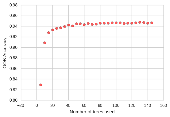
Out of bag accuracy sits near 0.83 at five trees, passes 0.92 by twenty, and is flat around 0.945 from roughly forty on. I set 25 trees and left it there; reading the chart again, 50 would have been the better call.
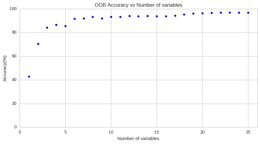
One feature gets about 43 percent. Two gets 70, three gets 84, and five gets roughly 85. Six jumps to 91.5, ten reaches 93, and it takes the full 25 to creep back toward the 96.5 the whole model had.
Eighty five percent at five features. The model I settle on also uses five features, and it scores 94.50. Those cannot be the same five.
Correlated features split their importance
The README in repo describes how I built a model, drop the features with low importance, retrain on what is left, read the new importances, repeat till final model. Two rankings taken at different points in that loop disagree, and the correlation blocks from earlier are why. Importance in a random forest is credit for splits, and correlated features divide that credit between them. A feature can score low in the full model only because four near copies of it are splitting the credit. Drop most of the block and the one left inherits the whole score. So the ranking reshuffles after every trim, and the five that finish on top are five the first pass had no way to find.
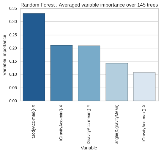
The final five:
angle(X,gravityMean)tGravityAcc-mean()-YtGravityAcc-min()-XtGravityAcc-max()-XtBodyAcc-mad()-X
tBodyAcc-mad()-X tops that chart at about 0.33, then tGravityAcc-min()-X and tGravityAcc-mean()-Y near 0.21, angle(X,gravityMean) at 0.14 and tGravityAcc-max()-X at 0.11. The best of the 561 carried 0.034, so selection concentrated importance about tenfold, and it concentrated it on the one motion feature in the set. The four gravity orientation features carry the other 0.67 between them. That division reads sensibly after the fact. Gravity points a fixed way relative to the world, so the angle between phone and gravity reads posture, and posture is most of what separates sitting from standing from laying. tBodyAcc-mad()-X is the mean absolute deviation of body acceleration along one axis, roughly how much the phone is being shaken.
The forest picked these features, not a biomechanics argument. The posture story came afterwards, as a check that the selection was not absurd. It passed, and it did none of the selecting.
Where the 124 errors live
Five features, 25 trees, and now the test set for the first time. 94.50 percent out of bag on the training records, 94.37 percent on the 2206 held out ones, which is 2082 correct. I trained a Support Vector Machine on the same five features for comparison.
| Random-Forest | SVM | |
|---|---|---|
| Train | 94.50% (oob) | 83.48% |
| Test | 94.37% | 82.37% |
The forest’s score is the out of bag score, so it is already a held out number; the SVM’s is resubstitution accuracy, the model graded on the rows it was fit on. The comparison that means something is out of bag against test, and for the forest those land 0.13 points apart. The SVM loses by about 12 points on the test set.
124 test records come out wrong, and they are heavily clustered. 86 of them are inside the walking trio, where walk, walkup and walkdown trade windows in every direction. Another 38 are the sitting and standing pair: 17 sitting windows read as standing, 21 standing windows read as sitting. Both are upright and motionless, so the four gravity features see almost the same thing in each, and no other pair trades as many windows. Laying is the one activity with no errors at all, 423 out of 423, which follows from it being the only posture where gravity runs along a different phone axis entirely.
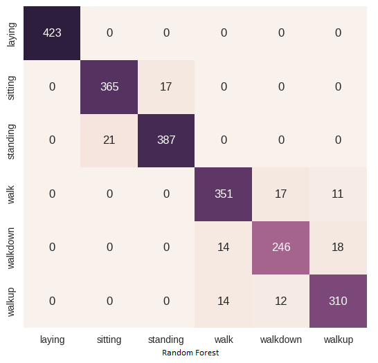
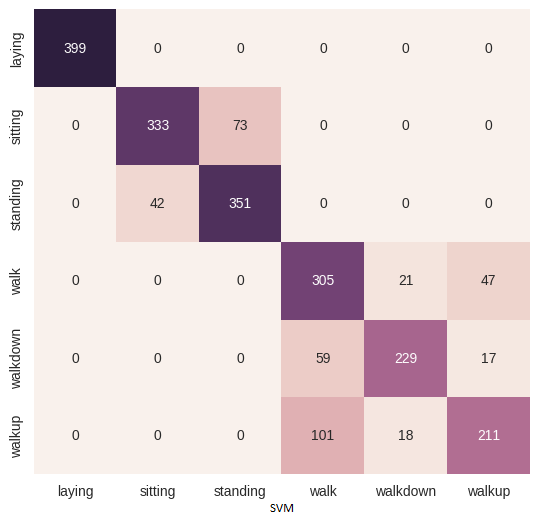
The SVM’s failures are the same failures at higher volume. Its sitting and standing confusion runs to 115 records against the forest’s 38, and it sends 101 walkup windows to walk where the forest sends 14. Laying it also gets clean, 399 of them.
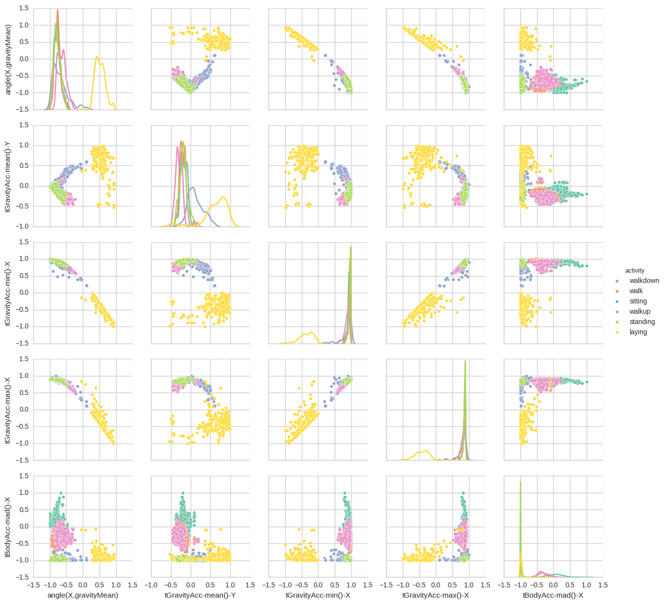
tBodyAcc-mad()-X pins the three still activities near -1 while the three walking activities spread across its range.Laying pulls away on the gravity pairs. Sitting and standing sit on top of each other in every panel that contains them, which is where the 38 errors come from.
The gap I did not measure
Five numbers and 25 trees are cheap enough to run on the phone continuously, which is the only place activity recognition is useful, and computing all 561 every 2.56 seconds is not something I would ask of a battery.
There were two limits in this post :
The first is the split. The 0.13 point gap between 94.50 out of bag and 94.37 on test says the five feature model is not memorizing individual training windows. It says nothing about a new person, because there is no new person in the file: the split is by record, the same 21 subjects sit on both sides, and with 50 percent window overlap a fair number of test records are near twins of training ones. The UCI subject-wise split would answer it. I did not re-run it, so I am not going to put a number on how far the accuracy would fall.
The second is the population. 21 volunteers between 19 and 48, six activities, one phone position. I trusted a random forest not to overfit here because the training data is reasonably balanced, and the class counts up top say it is. Move to a population that skews, an age band these volunteers never covered, a gait the sensors never saw, a phone in a pocket instead of at the waist, and that assumption is the first thing I would stop trusting.
References
Random Forest:
- https://www.stat.berkeley.edu/~breiman/RandomForests/cc_home.htm
- http://scikit-learn.org/stable/modules/ensemble.html#forest
- https://en.wikipedia.org/wiki/Random_forest
SVM:
- http://scikit-learn.org/stable/modules/svm.html
- https://en.wikipedia.org/wiki/Support_vector_machine
OOB Score:
- https://www.stat.berkeley.edu/~breiman/RandomForests/cc_home.htm#ooberr
- http://scikit-learn.org/stable/auto_examples/ensemble/plot_ensemble_oob.html
UCI-ML dataset location:
Scikit-Learn:
GitHub Page: