You wrote the obvious thing. A column of a million numbers, and you needed their sum, so you reached for the loop your fingers already know:

total = 0.0
for x in data:
    total += x

It returned the right answer in about 9.8 ms. Then you replaced three lines with one, data.sum(), and got the same sum to every digit you cared about in 0.16 ms. (Not bitwise identical, as it turns out, for a reason I owe you at the end.) One line of intent, sixty times faster: 60x at $n = 1{,}000{,}000$.

That gap stops you. Nothing about the loop looked wasteful. It did one add per number. The least work the sum could possibly require. So where did the other fifty-nine sixtieths go?

It went to bookkeeping. The loop spent almost all of its time not adding. Every iteration, the interpreter fetched a boxed Python float, checked its type, unboxed it, dispatched + through its dynamic-dispatch machinery, re-boxed the result, and advanced the iterator. A million times over. The arithmetic you actually wanted was a rounding error in the cost. data.sum() did the same million adds in one compiled C loop over a contiguous buffer and paid that overhead exactly once.

A Python loop over a million numbers is you doing the CPU’s bookkeeping by hand. That is the thing I kept poking at. So I ran six of these as paired benchmarks, the loop I’d write by hand against the whole-array call, and the speedups land anywhere from 3x to 382x. That spread isn’t noise. It’s a precise story about how much bookkeeping each hand-off recovers, and where it stops paying. 60x for a sum is the middle of it. The same logic bottoms out at 3x for a filter and tops out at 382x for a dot.

I’m going to climb that spread as a ladder. Each rung is a bigger lever than the one below. Start at the bare loop. Then a whole-array reduction. Then broadcasting. Then @, the dot. The thing that actually predicts every win, compute per byte moved, sits at the top. I’ll name it last, once the rungs underneath have earned it, not hand it to you as a thesis up front.

(Originally written in 2017; rewritten and re-benchmarked in 2022. The prose and the numbers below are from the 2022 pass.)

A note on the numbers, so you can weigh them. Every figure is a paired benchmark on one machine: the loop and the array call timed against each other, best of several timeit runs after a warmup. I report them relative to each other, never in absolute hardware terms, because the ratio is the portable part. The headline bar chart and the size sweep are two independent runs, so the same operation’s $n = 10^6$ figure differs by about $1\times$ between them. I’ll flag it where it shows.

At a glance. Six operations, each timed as a hand-written Python loop against its one-line whole-array NumPy call at $n = 10^6$. The speedups span 3x to 382x, and the spread is not noise: it tracks how much interpreter bookkeeping each call recovers and where the memory-bandwidth ceiling caps it. Two rules fall out, and they’re the whole post: vectorize once $n$ is in the thousands (below that a loop is fine, sometimes faster), and your ceiling is memory bandwidth unless @ takes you to BLAS - compute-per-byte predicts the win every time.

Rung 0: the loop is doing the CPU’s bookkeeping

Start at the bottom. Look again at what for x in data: total += x executes, per element. It fetches a PyObject pointer, type-checks it, unboxes it to a machine number, adds through PyNumber_Add’s dynamic dispatch (because Python can’t assume + means float addition until it inspects the operands), re-boxes the result into a fresh heap object, and advances the iterator. The add you cared about is one cheap instruction wearing a dozen expensive ones.

The costs aren’t one thing. So it helps to name them:

  1. Bytecode dispatch through the CPython evaluation loop. Every operation is an interpreted instruction.
  2. Boxing and unboxing, plus the dynamic type dispatch that decides what + even means this time around.
  3. Pointer-chasing. A Python list isn’t a block of numbers; it’s a block of pointers to scattered heap objects. Each element is a separate cache-unfriendly dereference. (A NumPy array, by contrast, is one contiguous block of raw numbers.)
  4. Iterator and bounds overhead on every step.

Here are the two snippets side by side:

import numpy as np

rng = np.random.default_rng(0)
data = rng.standard_normal(1_000_000)

# the loop: interpreter does the bookkeeping, n times
total = 0.0
for x in data:
    total += x

# the array call: one typed C loop over a contiguous buffer
total = data.sum()
One element at a time versus one call over the buffer A buffer of eight contiguous cells, shown twice. In the Python loop the interpreter visits one cell at a time, paying type-check, unbox, add and rebox on each, repeated n times. In the whole-array version one typed C pass sweeps the entire buffer once.
A million Python iterations means a million rounds of type-checking and (un)boxing, paid per element by the interpreter. One whole-array call hands the buffer to a single typed C loop and pays that overhead exactly once.

Here is the part to internalize. You are not removing the loop. The million adds still happen. You moved the loop out of the interpreter and into compiled C, where the types are known once, the buffer is contiguous, and the dispatch is paid a single time.

Put a rough size on it. The sum loop’s 9.8 ms over a million elements is about 9.8 ns each, and essentially all of that is bookkeeping, since the bare float add is sub-nanosecond. The array call collapses that 9.8 ns down toward the cost of streaming one number from memory. SIMD (the CPU doing several adds per instruction) is a real effect on top of this, but it’s second-order; the first-order win is interpreter-to-C. Vectorization doesn’t change the loop’s $O(n)$. There are still $n$ adds. It collapses the constant in front of the $n$.

That’s the lowest rung. Every rung above is this same trade under a different shape of work. Climb.

The array call has a fixed cost too

Before the climb, one thing about the rung itself. The array call has its own fixed price. Before NumPy touches your data it parses arguments, resolves dtypes and shapes, works out broadcasting, allocates an output buffer, and sets up the ufunc and its iterator. That bill is paid once per call, no matter how big the array is. Which means at small enough $n$ the loop wins outright. For a*b + c at $n = 10$, the vectorized version clocks 0.9x: below parity, slower than the loop.

One expression captures the behaviour:

\[\text{speedup}(n) = \frac{n \cdot c_{\text{py}}}{C_{\text{fixed}} + n \cdot c_{\text{elem}}(n)}\]

$C_{\text{fixed}}$ is that per-call setup. $c_{\text{py}}$ is the loop’s per-element cost, far larger than NumPy’s. The term that does the real work is $c_{\text{elem}}(n)$, NumPy’s cost per element, which is not a constant. While the working set fits in cache it’s small and roughly flat; once the arrays spill to main memory it rises toward the bandwidth-bound value. With $c_{\text{elem}}$ constant the formula could only climb and saturate. Let it vary with $n$ and the same formula predicts both the climb and the fall.

When $n$ is tiny, $C_{\text{fixed}}$ dominates the denominator and the speedup is flat and unimpressive. As $n$ grows the fixed cost amortizes and the ratio climbs. Then $c_{\text{elem}}(n)$ starts rising and pulls it back down.

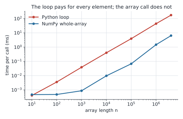
Time per call versus array length. The Python loop rises as a straight diagonal while the NumPy line stays nearly flat.
Time per call for a*b + c versus $n$. The loop is a clean diagonal, linear in $n$, exactly the per-element bookkeeping. The NumPy line is nearly flat until $n \approx 1000$: that floor is $C_{\text{fixed}}$, the fixed per-call overhead, before there's enough data to amortize it.

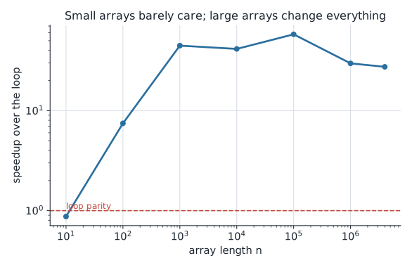
The size sweep for a*b + c tells the rest: 0.9x at $n=10$, 7.5x at 100, 44.6x at 1000, 41.3x at 10,000, a peak of 57.9x near 100,000, then back down to 29.7x at a million and 27.4x at four million.

Speedup versus array length. The curve starts low, climbs steeply to a peak, then settles to a lower plateau.
Speedup of the array call over the loop for a*b + c. Below the dashed $1\times$ parity line the loop wins. The curve climbs as $C_{\text{fixed}}$ amortizes, peaks at $\approx 58\times$ near $n = 10^5$ (the operands plus a hidden temporary still fit a fast cache level), then settles to $\approx 27\times$ once the arrays spill out of cache and the array path hits the memory-bandwidth ceiling.

That peak-then-settle shape catches people out: more data buys you less speedup at the top end. Near $n = 10^5$ the operands and the hidden temporary a*b still fit in a fast cache level, so $c_{\text{elem}}$ is near its floor and the array path runs near its best. Past that, the arrays exceed last-level cache, $c_{\text{elem}}$ climbs toward the rate at which memory can stream the data, and the speedup settles. The falloff is the array side slowing down, not the loop speeding up. The loop’s bottleneck is the interpreter, which never cared about your cache hierarchy at all.

So the win is biggest in the middle of the size range: past the fixed overhead, before the bandwidth wall. At a handful of elements the loop is fine, sometimes faster, and that’s the only regime where thinking in arrays doesn’t pay.

Rung 1: a reduction has an axis

Sum was the first rung. Now generalize it. Sum, mean, std, var, argmax, argmin, the statistical operations from any NumPy cheat-sheet, aren’t six separate tricks. They’re one pattern: a reduction collapses an axis. argmax and argmin fold right in, the reductions that return an index instead of a value, tracking the running best as they sweep.

I measured sum at 60x. The rest share the same single-pass reduction structure, so expect the same order of magnitude, with std and var a touch different because they do more arithmetic per element. The point isn’t a table of six numbers; it’s that one mental move covers all of them.

The upgrade for a loop-thinker is to stop asking “how do I loop over rows accumulating?” and start asking “which axis disappears?” On a 2-D array, axis=0 collapses the rows and leaves one value per column; axis=1 collapses the columns and leaves one value per row.

Summing over an axis collapses it A 3 by 4 array. Summing over axis 0 sends arrows down each column into a single row of four results, shape (4,). Summing over axis 1 sends arrows right along each row into a single column of three results, shape (3,). The axis you name is the one that disappears.
A reduction removes the axis it runs over: sum(axis=0) on a $(3,4)$ array returns shape $(4,)$, sum(axis=1) returns $(3,)$. The axis you name is the one that disappears. That is why a reduction is one keyword, not a hand-rolled accumulator plus an index.

The mnemonic that trips up everyone at first: the axis you name is the axis that vanishes.

X = rng.standard_normal((1000, 50))   # (n, d)
X.sum(axis=0)   # collapse the 1000 rows -> shape (50,), one value per column
X.sum(axis=1)   # collapse the 50 columns -> shape (1000,), one value per row

This is also why the loop was both slow and bug-prone: you were hand-rolling an accumulator, sometimes an index alongside it, that NumPy states as a single keyword.

One precision note, because the old cheat-sheets get it exactly backwards. Never pass dtype=np.float32 to a reduction; it down-casts the accumulator, and accumulating a million values in 32-bit loses accuracy fast. Integer sums up-cast the accumulator to int64 to dodge silent overflow.

Now the counter-case, because this rung is not flat. Cumulative sum is only 9x (loop 30 ms, array 3.4 ms), the second-smallest win in the set. A naive left-to-right scan is sequential, and that’s exactly what np.cumsum does: out[i] depends on out[i-1], one pass, one thread. Work-efficient parallel scans exist (Blelloch, Hillis-Steele), but NumPy doesn’t reach for one here, and the operation has to write a full $n$-element output, so it stays memory-bound coming and going.

np.cumsum(a)   # sequential left-fold + full n-element output -> only ~9x

That ceiling is telling you something true about how this operation is implemented, not a law of nature. Not every loop collapses to a fast one-liner. More of them do than you’d guess.

Rung 2: broadcasting is shape, not loops

This is the hard rung. A loop-thinker accepts whole-array sum and add quickly, because they map one-to-one onto a loop you can already picture. Broadcasting breaks the model: the shapes differ, and NumPy silently invents the missing axis. So look at the picture before the rule.

A size-1 axis stretches to fit, and no data is copied A (3,1) column plus a (1,4) row equals a (3,4) grid. The column's single column is reused across four columns; the row's single row is reused across three rows. The dashed ghost cells are virtual: read repeatedly along a stride-0 axis, never copied. Only the result is materialized.
Broadcasting aligns shapes from the right; any axis of length 1 is reused along the other operand as a stride-0 step, read repeatedly without ever being copied. Subtracting a row of column means from a matrix is $(n,d) - (1,d)$: the means are read $n$ times, but only the result is materialized.

That stretch is the whole mechanism: a (3,1) column and a (1,4) row combine into a (3,4) grid, each operand reused along the axis it’s missing. Now the concrete case. Z-score a matrix by column: subtract each column’s mean, divide by its standard deviation. The loop is genuinely ugly. An outer pass over columns to compute statistics, an inner pass over rows to apply them.

# loop-first: nested, and easy to get the indexing wrong
out = np.empty_like(X)
for j in range(X.shape[1]):
    col = X[:, j]
    m = col.mean()
    s = col.std()
    for i in range(X.shape[0]):
        out[i, j] = (X[i, j] - m) / s

The array form is one line, and it is not guessable from the loop:

(X - X.mean(axis=0)) / X.std(axis=0)   # (n, d) - (1, d) -> (n, d)

That’s 35x (loop 169 ms, array 4.8 ms). Read the shapes: X.mean(axis=0) is (d,), treated as (1, d), and stretched down across all $n$ rows.

The rule, stated as an algorithm: compare shapes from the trailing (rightmost) axis; a missing leading axis is treated as length 1; two dimensions are compatible if they’re equal or one of them is 1, and a size-1 axis is stretched to match. The example that kills the naive “left-align the shapes” intuition: (2,3) with (3,) succeeds (the 3s line up on the right), but (2,3) with (2,) fails, even though left-alignment would wrongly predict it works.

The mechanism that makes this cheap is the lever I keep circling: a stretched axis is a stride-0 axis. The iterator re-reads the same memory address as it walks that dimension. Broadcasting does not copy or tile the operand; the result is materialized, the operand is not. Subtracting a row of column means from a matrix is (n,d) - (1,d): the means are read $n$ times, allocated once.

Notice this couples the two rungs you just climbed. Reduce along an axis to get the means, then broadcast back along that same axis to subtract them. You run the one axis in both directions.

Two things to keep straight. Vectorized ops return a new array: b = a + c does not mutate a; there’s no out[i] = ... happening in place. And broadcasting is elementwise-bound, so expect elementwise-class speedups (tens of x), not the BLAS-class numbers one rung up.

A half-rung: masks replace the if inside the loop

Filtering is broadcasting’s smaller cousin, and it’s worth a stop because of how little it wins. The loop-thinker’s filter is a branch and a growing list:

keep = []
for x in data:
    if x > 0:
        keep.append(x)

Don’t jump straight to data[data > 0]. Build the model first. Start with the comparison alone:

mask = data > 0     # a boolean ARRAY, same shape as data, not a scalar
data[mask]          # gather the True positions

Here data > 0 doesn’t return a single True/False; it returns a whole boolean array of the same shape, one flag per element. Hold that idea and the rest of NumPy’s selection vocabulary opens up: mask.sum() counts the matches, np.where(mask, a, b) chooses elementwise.

And here’s the smallest number in the post: filter is 3.2x (loop 16 ms, array 5.0 ms). It’s the most instructive result here, not the weakest, because of why it’s small. data > 0 allocates a full $n$-byte boolean mask. Boolean indexing then counts the True entries to size the output, allocates it, and makes a second pass to gather the matching elements. Multiple memory passes, two heap allocations, all bandwidth-bound, and almost no arithmetic to amortize. The interpreter-to-C advantage is real, but here it has nothing to amplify.

That gap is the first time the top rung shows its face. Sum and dot do a lot of arithmetic per byte they touch, so they win big. Filter is nearly pure byte-moving, so it wins modestly. Same library, same trick, opposite ends of the spread. And note 3.2x is still a 3x speedup, and it deletes the bug-prone append loop, so filter is worth vectorizing even where the ratio looks unexciting.

One last fact to carry forward: boolean (and fancy integer) indexing returns a copy, whereas slicing returns a view. Slices like s[::-1], x[:, 1:3], and .T share memory with the original, so mutating a view writes through to the parent. The robust test for whether two arrays share storage is np.shares_memory(a, b), not a.base is b.

Rung 3: the @ operator is a different machine

Top of the ladder. The old cheat-sheets conflate two products. There’s the elementwise (Hadamard) product a * b, same shape in, same shape out, a single ufunc, elementwise-bound. And there’s the dot/matmul a @ b, which contracts over a shared axis. The clean way to choose: ask what the loop body is. One multiply per cell? That’s *. A sum of products over a shared axis? That’s @.

a * b   # Hadamard: one multiply per element, shapes match, elementwise class
a @ b   # dot: sum of products over the shared axis -> a scalar

a * b is one ufunc and lands in the same elementwise class as a*b + c, so expect tens of x, not BLAS numbers (I measured the combined a*b + c at 28x; a bare a*b is the same class). Use @ as the idiom. np.dot is the legacy spelling, fine for 1-D and 2-D, but it diverges from @ for higher dimensions, so don’t treat them as interchangeable.

The dot product is the biggest win in the set: 382x (loop 27.5 ms, array 0.072 ms). It’s fast for a different reason than everything above. @ hands off to a BLAS kernel that’s been tuned for decades: register-blocked, cache-tiled, multi-accumulator, fully SIMD and FMA’d, often multi-threaded. You’re not escaping the interpreter so much as renting an optimized numerical library, which is why dot sits an order of magnitude past every ufunc.

Two things bound that 382x. First, it’s contiguous, same-dtype operands; strided or mixed-dtype inputs can fall off the fast BLAS path entirely. Second, part of the ratio is the baseline being heavier: the loop-dot does both a multiply and a running-sum per element, more work per step than the elementwise loop. So the clean decomposition is this. The elementwise loop alone gave about 28x of interpreter-to-C. The extra factor up to 382x is BLAS plus that heavier per-step baseline, not “more vectorization.” A roofline says the same thing without the loop: a dot reduces to a scalar, so it has high arithmetic intensity and runs compute-bound near peak, while a*b + c has to write an $n$-element output and runs bandwidth-bound. Output size and arithmetic-per-byte predict the ranking, not “is it vectorized.”

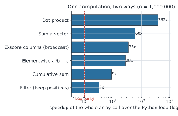
Horizontal bar chart on a log axis ranking the speedup of six whole array operations over their Python loops.
All six operations on one log axis at $n = 10^6$. Dot (BLAS, compute-bound) tops out at $382\times$; filter (memory-bound, almost no arithmetic) sits at the bottom near $3\times$. The elementwise bar reads $28\times$ here; the size sweep in Figure 3 puts the same op at $29.7\times$ for $n = 10^6$, the $\approx 1\times$ gap being the two independent runs. Nothing dips below the dashed $1\times$ parity line at this size, but recall Figure 3, where the same op fell to $0.9\times$ at $n = 10$.

A common assumption to drop: a*b + c does not fuse into a single pass by default. NumPy evaluates it as two ufuncs, multiply then add, with a full $n$-element temporary in between. So at large $n$ the expression briefly holds a, b, c, the temporary, and the result in memory at once, which is the real reason large-$n$ elementwise settles toward 27x instead of holding 58x. If the footprint bites, reach for in-place ops (np.multiply(a, b, out=a); a += c), an explicit out= buffer, or numexpr, which genuinely fuses the expression and skips the temporary. The irony: the Python loop allocates no large temporary at all. Vectorize-everything carries a real memory-footprint tradeoff, and it’s fair to say so plainly.

And the floating-point caveat I promised in the lede. FP addition isn’t associative, so the loop, np.sum, and a BLAS dot can disagree in the last bits; pairwise, blocked, and FMA orderings round differently. np.sum has used pairwise summation since NumPy 1.9, and its error grows like $O(\varepsilon \log n)$ instead of the $O(\varepsilon n)$ of a naive left-fold, so it is both faster and more accurate than the loop. Over a million standard-normal draws the left-fold loop and pairwise np.sum agree to about fifteen significant digits but not the last one, which is why the lede said “same to every digit you cared about” rather than “identical.” The array result is usually more accurate than your left-fold, not bitwise equal to it. So for a reduction or a dot, never say “same computation, just faster”; it’s the same math up to reassociation.

The top rung, named at last

Now I can name the lever the whole ladder was climbing toward: vectorization’s win scales with compute per byte moved. Sum and dot do a lot of arithmetic per byte they touch, so they win big. Filter is nearly pure byte-moving, so it wins modestly. Compute per byte runs the entire 3x-to-382x range you’ve watched unfold rung by rung.

It’s not my lever alone, either. “NumPy is the foundation upon which the scientific Python ecosystem is constructed.” That’s the verdict of the 2020 Nature paper written by the people who maintain it, and it reads less like a boast once you count what sits on top. Every pandas join, every scikit-learn fit, every SciPy solve is arithmetic running over a NumPy array. PyTorch and TensorFlow keep their own tensors but borrowed its array model. The library is pulled off PyPI on the order of a billion times a month, and more than a hundred thousand packages there name it as a dependency. Every one of them is riding the same compute-per-byte lever, at ecosystem scale.

The shift isn’t “memorize the vectorized form of each loop.” It’s that you stop writing the loop and hoping it’s fast, and start asking what shape the operation is. A reduction asks which axis dies. A broadcast stretches one axis; a mask selects along one; a contraction sums products over the shared axis with @. Name the shape and you state the intent once, then hand the bookkeeping to C, or for @ to BLAS, to be paid once instead of $n$ times.

Two rules earned from the measurements, and they’re what to carry out the door. Vectorize when $n$ is large enough to amortize the call, thousands and up; below that a loop is fine and sometimes faster. And your ceiling is memory bandwidth, the 27x settle, unless @ takes you to BLAS, which is the 382x. Compute-per-byte predicts the win every time.

One lever sits past everything on this ladder. Vectorizing collapses the constant in front of the $n$: the same work, run in C instead of Python. Changing the math can collapse the $n$ itself. A double sum $\sum_{ij} x_i y_j$ rewritten as $(\sum_i x_i)(\sum_j y_j)$ drops from $O(n^2)$ to $O(n)$, a win no array call over the naive loop will ever match. This post climbed the first ladder; the second one starts where this one ends.

The loop was you doing the CPU’s bookkeeping by hand, one element at a time. Next time your fingers start typing for x in, stop and ask what shape the operation really is. The speedup you’d leave on the table was never about clever code. It was about refusing to hand-run a loop the machine was begging to run for you.

Every number above is paired and reproducible: the loop and the array call timed against each other on one machine, reported relative to each other. The repo has all six operations and the size sweep, so you can read the 3x-to-382x spread off the same compute-per-byte lever it came from, and see where the elementwise curve crests and falls back.

Browse the code and reproduce the benchmarks NumPy broadcasting docs